
4.16: Least Squares Approximation
- Page ID
- 197445
\( \newcommand{\vecs}[1]{\overset { \scriptstyle \rightharpoonup} {\mathbf{#1}} } \)
\( \newcommand{\vecd}[1]{\overset{-\!-\!\rightharpoonup}{\vphantom{a}\smash {#1}}} \)
\( \newcommand{\dsum}{\displaystyle\sum\limits} \)
\( \newcommand{\dint}{\displaystyle\int\limits} \)
\( \newcommand{\dlim}{\displaystyle\lim\limits} \)
\( \newcommand{\id}{\mathrm{id}}\) \( \newcommand{\Span}{\mathrm{span}}\)
( \newcommand{\kernel}{\mathrm{null}\,}\) \( \newcommand{\range}{\mathrm{range}\,}\)
\( \newcommand{\RealPart}{\mathrm{Re}}\) \( \newcommand{\ImaginaryPart}{\mathrm{Im}}\)
\( \newcommand{\Argument}{\mathrm{Arg}}\) \( \newcommand{\norm}[1]{\| #1 \|}\)
\( \newcommand{\inner}[2]{\langle #1, #2 \rangle}\)
\( \newcommand{\Span}{\mathrm{span}}\)
\( \newcommand{\id}{\mathrm{id}}\)
\( \newcommand{\Span}{\mathrm{span}}\)
\( \newcommand{\kernel}{\mathrm{null}\,}\)
\( \newcommand{\range}{\mathrm{range}\,}\)
\( \newcommand{\RealPart}{\mathrm{Re}}\)
\( \newcommand{\ImaginaryPart}{\mathrm{Im}}\)
\( \newcommand{\Argument}{\mathrm{Arg}}\)
\( \newcommand{\norm}[1]{\| #1 \|}\)
\( \newcommand{\inner}[2]{\langle #1, #2 \rangle}\)
\( \newcommand{\Span}{\mathrm{span}}\) \( \newcommand{\AA}{\unicode[.8,0]{x212B}}\)
\( \newcommand{\vectorA}[1]{\vec{#1}} % arrow\)
\( \newcommand{\vectorAt}[1]{\vec{\text{#1}}} % arrow\)
\( \newcommand{\vectorB}[1]{\overset { \scriptstyle \rightharpoonup} {\mathbf{#1}} } \)
\( \newcommand{\vectorC}[1]{\textbf{#1}} \)
\( \newcommand{\vectorD}[1]{\overrightarrow{#1}} \)
\( \newcommand{\vectorDt}[1]{\overrightarrow{\text{#1}}} \)
\( \newcommand{\vectE}[1]{\overset{-\!-\!\rightharpoonup}{\vphantom{a}\smash{\mathbf {#1}}}} \)
\( \newcommand{\vecs}[1]{\overset { \scriptstyle \rightharpoonup} {\mathbf{#1}} } \)
\(\newcommand{\longvect}{\overrightarrow}\)
\( \newcommand{\vecd}[1]{\overset{-\!-\!\rightharpoonup}{\vphantom{a}\smash {#1}}} \)
\(\newcommand{\avec}{\mathbf a}\) \(\newcommand{\bvec}{\mathbf b}\) \(\newcommand{\cvec}{\mathbf c}\) \(\newcommand{\dvec}{\mathbf d}\) \(\newcommand{\dtil}{\widetilde{\mathbf d}}\) \(\newcommand{\evec}{\mathbf e}\) \(\newcommand{\fvec}{\mathbf f}\) \(\newcommand{\nvec}{\mathbf n}\) \(\newcommand{\pvec}{\mathbf p}\) \(\newcommand{\qvec}{\mathbf q}\) \(\newcommand{\svec}{\mathbf s}\) \(\newcommand{\tvec}{\mathbf t}\) \(\newcommand{\uvec}{\mathbf u}\) \(\newcommand{\vvec}{\mathbf v}\) \(\newcommand{\wvec}{\mathbf w}\) \(\newcommand{\xvec}{\mathbf x}\) \(\newcommand{\yvec}{\mathbf y}\) \(\newcommand{\zvec}{\mathbf z}\) \(\newcommand{\rvec}{\mathbf r}\) \(\newcommand{\mvec}{\mathbf m}\) \(\newcommand{\zerovec}{\mathbf 0}\) \(\newcommand{\onevec}{\mathbf 1}\) \(\newcommand{\real}{\mathbb R}\) \(\newcommand{\twovec}[2]{\left[\begin{array}{r}#1 \\ #2 \end{array}\right]}\) \(\newcommand{\ctwovec}[2]{\left[\begin{array}{c}#1 \\ #2 \end{array}\right]}\) \(\newcommand{\threevec}[3]{\left[\begin{array}{r}#1 \\ #2 \\ #3 \end{array}\right]}\) \(\newcommand{\cthreevec}[3]{\left[\begin{array}{c}#1 \\ #2 \\ #3 \end{array}\right]}\) \(\newcommand{\fourvec}[4]{\left[\begin{array}{r}#1 \\ #2 \\ #3 \\ #4 \end{array}\right]}\) \(\newcommand{\cfourvec}[4]{\left[\begin{array}{c}#1 \\ #2 \\ #3 \\ #4 \end{array}\right]}\) \(\newcommand{\fivevec}[5]{\left[\begin{array}{r}#1 \\ #2 \\ #3 \\ #4 \\ #5 \\ \end{array}\right]}\) \(\newcommand{\cfivevec}[5]{\left[\begin{array}{c}#1 \\ #2 \\ #3 \\ #4 \\ #5 \\ \end{array}\right]}\) \(\newcommand{\mattwo}[4]{\left[\begin{array}{rr}#1 \amp #2 \\ #3 \amp #4 \\ \end{array}\right]}\) \(\newcommand{\laspan}[1]{\text{Span}\{#1\}}\) \(\newcommand{\bcal}{\cal B}\) \(\newcommand{\ccal}{\cal C}\) \(\newcommand{\scal}{\cal S}\) \(\newcommand{\wcal}{\cal W}\) \(\newcommand{\ecal}{\cal E}\) \(\newcommand{\coords}[2]{\left\{#1\right\}_{#2}}\) \(\newcommand{\gray}[1]{\color{gray}{#1}}\) \(\newcommand{\lgray}[1]{\color{lightgray}{#1}}\) \(\newcommand{\rank}{\operatorname{rank}}\) \(\newcommand{\row}{\text{Row}}\) \(\newcommand{\col}{\text{Col}}\) \(\renewcommand{\row}{\text{Row}}\) \(\newcommand{\nul}{\text{Nul}}\) \(\newcommand{\var}{\text{Var}}\) \(\newcommand{\corr}{\text{corr}}\) \(\newcommand{\len}[1]{\left|#1\right|}\) \(\newcommand{\bbar}{\overline{\bvec}}\) \(\newcommand{\bhat}{\widehat{\bvec}}\) \(\newcommand{\bperp}{\bvec^\perp}\) \(\newcommand{\xhat}{\widehat{\xvec}}\) \(\newcommand{\vhat}{\widehat{\vvec}}\) \(\newcommand{\uhat}{\widehat{\uvec}}\) \(\newcommand{\what}{\widehat{\wvec}}\) \(\newcommand{\Sighat}{\widehat{\Sigma}}\) \(\newcommand{\lt}{<}\) \(\newcommand{\gt}{>}\) \(\newcommand{\amp}{&}\) \(\definecolor{fillinmathshade}{gray}{0.9}\)- Find the least squares solution for an inconsistent system.
- Apply the least squares approximate to find the regression line given a collection of points.
It should not be surprising to hear that many problems do not have a perfect solution, and in these cases the objective is always to try to do the best possible. For example what does one do if there are no solutions to a system of linear equations \(A\vec{x}=\vec{b}\)? It turns out that what we do is find \(\vec{x}\) such that \(A\vec{x}\) is as close to \(\vec{b}\) as possible. A very important technique that follows from orthogonal projections is that of the least square approximation, and allows us to do exactly that.
We begin with a lemma.
Recall that we can form the image of an \(m \times n\) matrix \(A\) by \(\mathrm{im}\left( A\right) = \left\{ A\vec{x} : \vec{x} \in \mathbb{R}^n \right\}\). Rephrasing Theorem \(\PageIndex{4}\) using the subspace \(W=\mathrm{im}\left( A\right)\) gives the equivalence of an orthogonality condition with a minimization condition. The following picture illustrates this orthogonality condition and geometric meaning of this theorem.
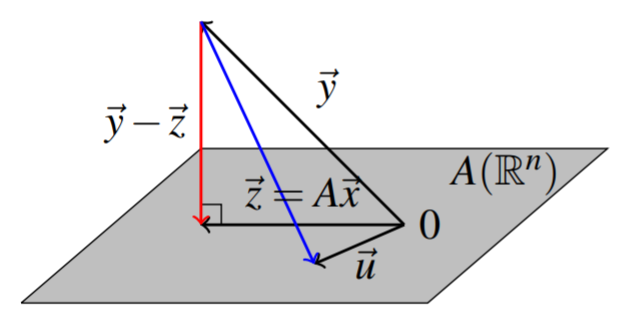
Let \(\vec{y}\in \mathbb{R}^{m}\) and let \(A\) be an \(m\times n\) matrix.
Choose \(\vec{z}\in W= \mathrm{im}\left( A\right)\) given by \(\vec{z} = \mathrm{proj}_{W}\left( \vec{y}\right)\), and let \(\vec{x} \in \mathbb{R}^{n}\) such that \(\vec{z}=A\vec{x}\).
Then
- \(\vec{y} - A\vec{x} \in W^{\perp}\)
- \( \| \vec{y} - A\vec{x} \| < \| \vec{y} - \vec{u} \| \) for all \(\vec{u} \neq \vec{z} \in W\)
We note a simple but useful observation.
Let \(A\) be an \(m\times n\) matrix. Then \[A\vec{x} \cdot \vec{y} = \vec{x}\cdot A^T\vec{y}\nonumber \]
- Proof
-
This follows from the definitions: \[A\vec{x} \cdot \vec{y}=\sum_{i,j}a_{ij}x_{j} y_{i} =\sum_{i,j}x_{j} a_{ji} y_{i}= \vec{x} \cdot A^T\vec{y}\nonumber \]
The next corollary gives the technique of least squares.
A specific value of \(\vec{x}\) which solves the problem of Theorem \(\PageIndex{5}\) is obtained by solving the equation \[A^TA\vec{x}=A^T\vec{y}\nonumber \] Furthermore, there always exists a solution to this system of equations.
- Proof
-
For \(\vec{x}\) the minimizer of Theorem \(\PageIndex{5}\), \(\left( \vec{y}-A\vec{x}\right) \cdot A \vec{u} =0\) for all \(\vec{u} \in \mathbb{R}^{n}\) and from Lemma \(\PageIndex{1}\), this is the same as saying \[A^T\left( \vec{y}-A\vec{x}\right) \cdot \vec{u}=0\nonumber \] for all \(u \in \mathbb{R}^{n}.\) This implies \[A^T\vec{y}-A^TA\vec{x}=\vec{0}.\nonumber \] Therefore, there is a solution to the equation of this corollary, and it solves the minimization problem of Theorem \(\PageIndex{5}\).
Note that \(\vec{x}\) might not be unique but \(A\vec{x}\), the closest point of \(A\left(\mathbb{R}^{n}\right)\) to \(\vec{y}\) is unique as was shown in the above argument.
Consider the following example.
Find a least squares solution to the system \[\left[ \begin{array}{rr} 2 & 1 \\ -1 & 3 \\ 4 & 5 \end{array} \right] \left[ \begin{array}{c} x \\ y \end{array} \right] =\left[ \begin{array}{c} 2 \\ 1 \\ 1 \end{array} \right]\nonumber \]
Solution
First, consider whether there exists a real solution. To do so, set up the augmnented matrix given by \[\left[ \begin{array}{rr|r} 2 & 1 & 2 \\ -1 & 3 & 1 \\ 4 & 5 & 1 \end{array} \right]\nonumber \] The reduced row-echelon form of this augmented matrix is \[\left[ \begin{array}{rr|r} 1 & 0 & 0 \\ 0 & 1 & 0 \\ 0 & 0 & 1 \end{array} \right]\nonumber \]
It follows that there is no real solution to this system. Therefore we wish to find the least squares solution. The normal equations are \[\begin{aligned} A^T A \vec{x} &= A^T \vec{y} \\ \left[ \begin{array}{rrr} 2 & -1 & 4 \\ 1 & 3 & 5 \end{array} \right] \left[ \begin{array}{rr} 2 & 1 \\ -1 & 3 \\ 4 & 5 \end{array} \right] \left[ \begin{array}{c} x \\ y \end{array} \right] &=\left[ \begin{array}{rrr} 2 & -1 & 4 \\ 1 & 3 & 5 \end{array} \right] \left[ \begin{array}{c} 2 \\ 1 \\ 1 \end{array} \right]\end{aligned}\] and so we need to solve the system \[\left[ \begin{array}{rr} 21 & 19 \\ 19 & 35 \end{array} \right] \left[ \begin{array}{c} x \\ y \end{array} \right] =\left[ \begin{array}{r} 7 \\ 10 \end{array} \right]\nonumber \] This is a familiar exercise and the solution is \[\left[ \begin{array}{c} x \\ y \end{array} \right] =\left[ \begin{array}{c} \frac{5}{34} \\ \frac{7}{34} \end{array} \right]\nonumber \]
Consider another example.
Find a least squares solution to the system \[\left[ \begin{array}{rr} 2 & 1 \\ -1 & 3 \\ 4 & 5 \end{array} \right] \left[ \begin{array}{c} x \\ y \end{array} \right] =\left[ \begin{array}{c} 3 \\ 2 \\ 9 \end{array} \right]\nonumber \]
Solution
First, consider whether there exists a real solution. To do so, set up the augmnented matrix given by \[\left[ \begin{array}{rr|r} 2 & 1 & 3 \\ -1 & 3 & 2 \\ 4 & 5 & 9 \end{array} \right]\nonumber\] The reduced row-echelon form of this augmented matrix is \[\left[ \begin{array}{rr|r} 1 & 0 & 1 \\ 0 & 1 & 1 \\ 0 & 0 & 0 \end{array} \right]\nonumber \]
It follows that the system has a solution given by \(x=y=1\). However we can also use the normal equations and find the least squares solution. \[\left[ \begin{array}{rrr} 2 & -1 & 4 \\ 1 & 3 & 5 \end{array} \right] \left[ \begin{array}{rr} 2 & 1 \\ -1 & 3 \\ 4 & 5 \end{array} \right] \left[ \begin{array}{c} x \\ y \end{array} \right] =\left[ \begin{array}{rrr} 2 & -1 & 4 \\ 1 & 3 & 5 \end{array} \right] \left[ \begin{array}{r} 3 \\ 2 \\ 9 \end{array} \right]\nonumber \] Then \[\left[ \begin{array}{rr} 21 & 19 \\ 19 & 35 \end{array} \right] \left[ \begin{array}{c} x \\ y \end{array} \right] =\left[ \begin{array}{c} 40 \\ 54 \end{array} \right]\nonumber \]
The least squares solution is \[\left[ \begin{array}{c} x \\ y \end{array} \right] =\left[ \begin{array}{c} 1 \\ 1 \end{array} \right]\nonumber \] which is the same as the solution found above.
An important application of Corollary \(\PageIndex{1}\) is the problem of finding the least squares regression line in statistics. Suppose you are given points in the \(xy\) plane \[\left\{ \left( x_{1},y_{1}\right), \left( x_{2},y_{2}\right), \cdots, \left( x_{n},y_{n}\right) \right\}\nonumber \] and you would like to find constants \(m\) and \(b\) such that the line \(\vec{y}=m\vec{x}+b\) goes through all these points. Of course this will be impossible in general. Therefore, we try to find \(m,b\) such that the line will be as close as possible. The desired system is
\[\left[ \begin{array}{c} y_{1} \\ \vdots \\ y_{n} \end{array} \right] =\left[ \begin{array}{cc} x_{1} & 1 \\ \vdots & \vdots \\ x_{n} & 1 \end{array} \right] \left[ \begin{array}{c} m \\ b \end{array} \right]\nonumber \]
which is of the form \(\vec{y}=A\vec{x}\). It is desired to choose \(m\) and \(b\) to make
\[\left \| A\left[ \begin{array}{c} m \\ b \end{array} \right] -\left[ \begin{array}{c} y_{1} \\ \vdots \\ y_{n} \end{array} \right] \right \| ^{2}\nonumber \]
as small as possible. According to Theorem \(\PageIndex{5}\) and Corollary \(\PageIndex{1}\), the best values for \(m\) and \(b\) occur as the solution to
\[A^{T}A\left[ \begin{array}{c} m \\ b \end{array} \right] =A^{T}\left[ \begin{array}{c} y_{1} \\ \vdots \\ y_{n} \end{array} \right] ,\ \;\mbox{where}\; A=\left[ \begin{array}{cc} x_{1} & 1 \\ \vdots & \vdots \\ x_{n} & 1 \end{array} \right]\nonumber \]
Thus, computing \(A^{T}A,\)
\[\left[ \begin{array}{cc} \sum_{i=1}^{n}x_{i}^{2} & \sum_{i=1}^{n}x_{i} \\ \sum_{i=1}^{n}x_{i} & n \end{array} \right] \left[ \begin{array}{c} m \\ b \end{array} \right] =\left[ \begin{array}{c} \sum_{i=1}^{n}x_{i}y_{i} \\ \sum_{i=1}^{n}y_{i} \end{array} \right]\nonumber \]
Solving this system of equations for \(m\) and \(b\) (using Cramer’s rule for example) yields:
\[m= \frac{-\left( \sum_{i=1}^{n}x_{i}\right) \left( \sum_{i=1}^{n}y_{i}\right) +\left( \sum_{i=1}^{n}x_{i}y_{i}\right) n}{\left( \sum_{i=1}^{n}x_{i}^{2}\right) n-\left( \sum_{i=1}^{n}x_{i}\right) ^{2}}\nonumber \] and \[b=\frac{-\left( \sum_{i=1}^{n}x_{i}\right) \sum_{i=1}^{n}x_{i}y_{i}+\left( \sum_{i=1}^{n}y_{i}\right) \sum_{i=1}^{n}x_{i}^{2}}{\left( \sum_{i=1}^{n}x_{i}^{2}\right) n-\left( \sum_{i=1}^{n}x_{i}\right) ^{2}}.\nonumber \]
Consider the following example.
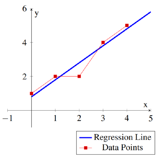
Find the least squares regression line \(y=mx+b\) for the following set of data points: \[\left\{ (0,1), (1,2), (2,2), (3,4), (4,5) \right\} \nonumber\]
Solution
In this case we have \(n=5\) data points and we obtain: \[\begin{array}{ll} \sum_{i=1}^{5}x_{i} = 10 & \sum_{i=1}^{5}y_{i} = 14 \\ \\ \sum_{i=1}^{5}x_{i}y_{i} = 38 & \sum_{i=1}^{5}x_{i}^{2} = 30\\ \end{array}\nonumber \] and hence \[\begin{aligned} m &= \frac{- 10 * 14 + 5*38}{5*30-10^2} = 1.00 \\ \\ b &= \frac{- 10 * 38 + 14*30}{5*30-10^2} = 0.80 \\\end{aligned}\]
The least squares regression line for the set of data points is: \[y = x+.8\nonumber \]
One could use this line to approximate other values for the data. For example for \(x=6\) one could use \(y(6)=6+.8=6.8\) as an approximate value for the data.
The following diagram shows the data points and the corresponding regression line.
One could clearly do a least squares fit for curves of the form \(y=ax^{2}+bx+c\) in the same way. In this case you want to solve as well as possible for \(a,b,\) and \(c\) the system \[\left[ \begin{array}{ccc} x_{1}^{2} & x_{1} & 1 \\ \vdots & \vdots & \vdots \\ x_{n}^{2} & x_{n} & 1 \end{array} \right] \left[ \begin{array}{c} a \\ b \\ c \end{array} \right] =\left[ \begin{array}{c} y_{1} \\ \vdots \\ y_{n} \end{array} \right]\nonumber \] and one would use the same technique as above. Many other similar problems are important, including many in higher dimensions and they are all solved the same way.