Section 2.3: Solving Equations - Advanced Techniques and Formulas

Be Prepared

We will rely heavily on these skills throughout this section.

• Find the LCD of \(\frac{5}{6}\) and \(\frac{1}{4}\)
• Solve \(6x+24=-2x+96\)
• Identify the reciprocal of \(\frac{2}{3}\)

Learning Objectives

Motivating Problem

You’re planning a road trip and you know the distance and your speed, but you want to figure out how long it will take. You’ve heard the formula is \(d=rt\), but the thing you don’t know is time.

So, how do you rewrite the formula to solve for the variable you actually care about?

Fun Fact

The formula \(E=mc^{2}\) became famous thanks to Einstein, but did you know solving it for \(m\) or \(c\) is just algebra? Rearranging formulas like this is precisely what scientists and engineers do every day to make predictions, design technology, and understand the universe—just with cooler variables!

The Goal

This section introduces strategies for solving more complex equations that involve fractions, decimals, or multiple steps. We’ll then continue building fluency with solving linear equations and learn how to clear messy-looking formulas into something manageable and useful.

Solve Equations with Fraction Coefficients

Let’s use the general strategy for solving linear equations introduced earlier to solve the equation, \(\frac{1}{8}x+\frac{1}{2}=\frac{1}{4}\).

To isolate the x term, subtract \(\frac{1}{2}\) from both sides.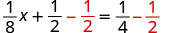
Simplify the left side.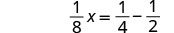
Change the constants to equivalent fractions with the LCD.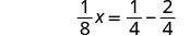
Subtract.
Multiply both sides by the reciprocal of \(\frac{1}{8}\).
Simplify.

This method worked fine, but many students do not feel very confident when they see all those fractions. So, we are going to show an alternate method to solve equations with fractions. This alternate method eliminates the fractions.

We will apply the Multiplication Property of Equality and multiply both sides of an equation by the least common denominator of all the fractions in the equation. The result of this operation will be a new equation, equivalent to the first, but without fractions. This process is called “clearing” the equation of fractions.

Let’s solve a similar equation, but this time use the method that eliminates the fractions.

Example 1

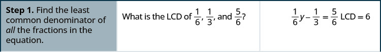
Solve: \(\frac{1}{6}y - \frac{1}{3} = \frac{5}{6}\)

Solution

Try It 1

Solve: \(\frac{1}{8}x + \frac{1}{2} = \frac{1}{4}\)

Answer

\(x = -2\)

Notice that in the previous exercise, once we cleared the equation of fractions, the equation resembled those we solved earlier in this chapter. We changed the problem to one we already knew how to solve! We then used the General Strategy for Solving Linear Equations.

STRATEGY TO SOLVE EQUATIONS WITH FRACTION COEFFICIENTS.

1. Find the least common denominator of all the fractions in the equation.
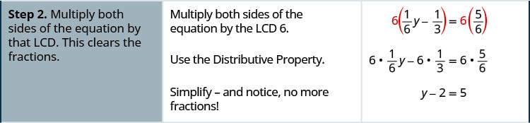
2. Multiply both sides of the equation by that LCD. This clears the fractions.
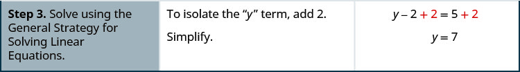
3. Solve using the General Strategy for Solving Linear Equations.

Example 2

Solve: \(6 = \frac{1}{2}v + \frac{2}{5}v - \frac{3}{4}v\)

Solution

We want to clear the fractions by multiplying both sides of the equation by the LCD of all the fractions in the equation.

Find the LCD of all fractions in the equation.
The LCD is 20.
Multiply both sides of the equation by 20.
Distribute.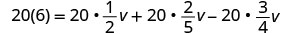
Simplify—notice, no more fractions!
Combine like terms.
Divide by 3.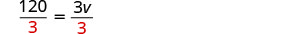
Simplify.
Check:
Let v=40.

Try It 2

Solve: \(-1 = \frac{1}{2}u + \frac{1}{4}u - \frac{2}{3}u\)

Answer

\(u = -12\)

In the next example, we again have variables on both sides of the equation.

Example 3

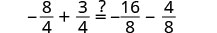
Solve: \(a + \frac{3}{4} = \frac{3}{8}a - \frac{1}{2}\)

Solution

Find the LCD of all fractions in the equation. The LCD is 8.
Multiply both sides by the LCD.
Distribute.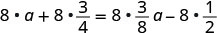
Simplify—no more fractions.
Subtract 3a3a from both sides.
Simplify.
Subtract 6 from both sides.
Simplify.
Divide by 5.
Simplify.
Check:
Let a=−2.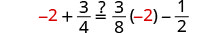

Try It 3

Solve: \(x + \frac{1}{3} = \frac{1}{6}x - \frac{1}{2}\)

Answer

\(x = -1\)

In the next example, we start by using the Distributive Property. This step clears the fractions right away.

Example 4

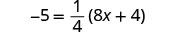
Solve: \(-5 = \frac{1}{4}(8x + 4)\)

Solution

Distribute.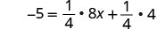
Simplify. Now there are no fractions.
Subtract 1 from both sides.
Simplify.
Divide by 2.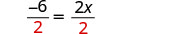
Simplify.
Check: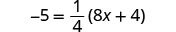
Let x=−3.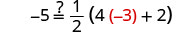

Try It 4

Solve: \(-11 = \frac{1}{2}(6p + 2)\)

Answer

\(p = -4\)

Example 5

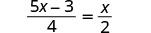
Solve: \(\frac{5x - 3}{4} = \frac{x}{2}\)

Solution

Multiply by the LCD, 4.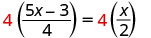
Simplify.
Collect the variables to the right.
Simplify.
Divide.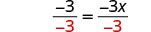
Simplify.
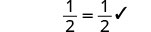
Check: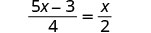
Let x=1.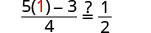

Try It 5

Solve: \(\frac{4y - 7}{3} = \frac{y}{6}\)

Answer

\(y = 2\)

Example 6

Solve: \(\frac{a}{6} + 2 = \frac{a}{4} + 3\)

Solution

Multiply by the LCD, 12.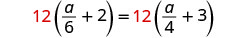
Distribute.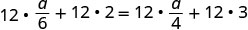
Simplify.
Collect the variables to the right.
Simplify.
Collect the constants to the left.
Simplify.
Check:
Let a=−12.

Try It 6

Solve: \(\frac{b}{10} + 2 = \frac{b}{4} + 5\)

Answer

\(b = -20\)

Solve Equations with Decimal Coefficients

Some equations have decimals in them. This kind of equation will occur when we solve problems dealing with money or percentages. But decimals can also be expressed as fractions. For example, \(0.3 = \frac{3}{10}\) and \(0.17 = \frac{17}{100}\). So, with an equation with decimals, we can use the same method we used to clear fractions—multiply both sides of the equation by the least common denominator.

Example 7

Solve: \(0.06x + 0.02 = 0.25x - 1.5\)

Solution

Look at the decimals and think of the equivalent fractions.

\(0.06 = \frac { 6 } { 100 } \quad 0.02 = \frac { 2 } { 100 } \quad 0.25 = \frac { 25 } { 100 } \quad 1.5 = 1 \frac { 5 } { 10 }\)

Notice, the LCD is 100.

By multiplying by the LCD, we will clear the decimals from the equation.

Multiply both side by 100.
Distribute.
Multiply, and now we have no more decimals.
Collect the variables to the right.
Simplify.
Collect the variables to the right.
Simplify.
Divide by 19.
Simplify.
Check: Let x=8

Try It 7

Solve: \(0.65k - 0.1 = 0.4k - 0.35\)

Answer

\(k = -1\)

The next example uses an equation that is typical of the money applications in the next chapter. Notice that we distribute the decimal before we clear all the decimals.

Example 8

Solve: \(0.25x + 0.05(x + 3) = 2.85\)

Solution

Distribute first.
Combine like terms.
To clear decimals, multiply by 100.
Distribute.
Subtract 15 from both sides.
Simplify.
Divide by 30.
Simplify.
Check it yourself by substituting x=9 into the original equation.

Try It 8

Solve: \(0.10d + 0.05(d -5) = 2.15\)

Answer

\(d = 16\)

Use the Distance, Rate, and Time Formula

One formula you will use often in algebra and in everyday life is the formula for distance traveled by an object moving at a constant rate. Rate is an equivalent word for “speed.” The basic idea of rate may already familiar to you. Do you know what distance you travel if you drive at a steady rate of 60 miles per hour for 2 hours? (This might happen if you use your car’s cruise control while driving on the highway.) If you said 120 miles, you already know how to use this formula!

DISTANCE, RATE, AND TIME

For an object moving at a uniform (constant) rate, the distance traveled, the elapsed time, and the rate are related by the formula:

\[\begin{array} {lllll}{ d = r t} &{\text { where }} &{ d} &{=} &{\text{distance}} \\ {} &{} &{ r} &{=} &{\text{rate}} \\{} &{} &{ t} &{=} &{\text{time}} \end{array}\nonumber\]

We will use the Strategy for Solving Applications that we used earlier in this chapter. When our problem requires a formula, we change Step 4. In place of writing a sentence, we write the appropriate formula. We write the revised steps here for reference.

SOLVE AN APPLICATION (WITH A FORMULA).

1. Read the problem. Make sure all the words and ideas are understood.
2. Identify what we are looking for.
3. Name what we are looking for. Choose a variable to represent that quantity.
4. Translate into an equation. Write the appropriate formula for the situation. Substitute in the given information.
5. Solve the equation using good algebra techniques.
6. Check the answer in the problem and make sure it makes sense.
7. Answer the question with a complete sentence.

You may want to create a mini-chart to summarize the information in the problem. See the chart in this first example.

Example 9

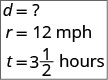
Jamal rides his bike at a uniform rate of 12 miles per hour for \(3\frac{1}{2}\) hours. What distance has he traveled?

Solution

Step 1. Read the problem.
Step 2. Identify what you are looking for.		distance traveled
Step 3. Name. Choose a variable to represent it.		Let d = distance.
Step 4. Translate: Write the appropriate formula.		\(d=rt\)
Substitute in the given information.		\(d = 12\cdot 3\frac{1}{2}\)
Step 5. Solve the equation.		\(d=42\text{ miles}\)
Step 6. Check
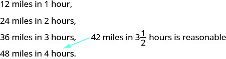
Does 42 miles make sense?
Jamal rides:
Step 7. Answer the question with a complete sentence.		Jamal rode 42 miles.

Try It 9

Trinh walked for \(2\frac{1}{3}\) hours at 3 miles per hour. How far did she walk?

Answer

7 miles

Example 10

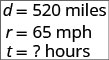
Rey is planning to drive from his house in San Diego to visit his grandmother in Sacramento, a distance of 520 miles. If he can drive at a steady rate of 65 miles per hour, how many hours will the trip take?

Solution

Step 1. Read the problem.
Step 2. Identify what you are looking for.	How many hours (time)
Step 3. Name. Choose a variable to represent it.	Let t = time.
Step 4. Translate. Write the appropriate formula.	\(d=rt\)
Substitute in the given information.	\(520 = 65t\)
Step 5. Solve the equation.	\(t = 8\)
Step 6. Check. Substitute the numbers into the formula and make sure the result is a true statement.
\(\begin{array}{lll} {d} &{=} &{rt} \\ {520} &{\stackrel{?}{=}} &{65\cdot 8}\\ {520} &{=} &{520\checkmark} \end{array}\)
Step 7. Answer the question with a complete sentence. Rey’s trip will take 8 hours.

Try It 10

Lee wants to drive from Phoenix to his brother’s apartment in San Francisco, a distance of 770 miles. If he drives at a steady rate of 70 miles per hour, how many hours will the trip take?

Answer

11 hours

Solve a Formula for a Specific Variable

You are probably familiar with some geometry formulas. A formula is a mathematical description of the relationship between variables. Formulas are also used in the sciences, such as chemistry, physics, and biology. In medicine, they are used for calculations for dispensing medicine or determining body mass index. Spreadsheet programs rely on formulas to make calculations. It is vital to be familiar with formulas and be able to manipulate them easily.

To solve a formula for a specific variable means to isolate that variable on one side of the equals sign with a coefficient of 1. All other variables and constants are on the other side of the equals sign. To see how to solve a formula for a specific variable, we will start with the distance, rate and time formula.

Example 11

Solve the formula \(d=rt\) for \(t\):

1. when \(d=520\) and \(r=65\)
2. in general

Solution

We will write the solutions side-by-side to demonstrate that solving a formula in general uses the same steps as when we have numbers to substitute.

1. when \(d=520\) and \(r=65\)		2. in general
Write the formula.	\(d=rt\)	Write the formula.	\(d=rt\)
Substitute.	\(520=65t\)
Divide, to isolate t.	\(\frac{520}{65} = \frac{65t}{65}\)	Divide, to isolate tt.	\(\frac{d}{r} = \frac{rt}{t}\)
Simplify.	\(8 = t\)	Simplify.	\(\frac{d}{r}=t\)

We say the formula \(t = \frac{d}{r}\) is solved for t.

Try It 11

Solve the formula \(d=rt\) for \(r\):

1. when \(d=780\) and \(t=12\)
2. in general

Answer

1. \(r = 65\)
2. \(r = \frac{d}{t}\)

Example 12

Solve the formula \(A = \frac{1}{2}bh\) for h:

1. when \(A = 90\) and \(b = 15\)
2. in general

Solution

1. when \(A = 90\) and \(b = 15\)		2. in general
Write the formula.		Write the formula.
Substitute.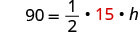
Clear the fractions.		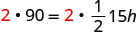Clear the fractions.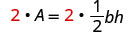
Simplify.		Simplify.
Solve for h.		Solve for hh.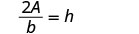

We can now find the height of a triangle if we know the area and the base by using the formula \(h = \frac{2A}{b}\)

Try It 12

Solve the formula \(A = \frac{1}{2}bh\) for h:

1. when \(A = 62\) and \(h = 31\)
2. in general

Answer

1. \(b = 4\)
2. \(b = \frac{2A}{h}\)

Later in this class, and in future algebra classes, you’ll encounter equations that relate two variables, usually x and y. You might be given an equation that is solved for y and need to solve it for x, or vice versa. In the following example, we’re given an equation with both x and y on the same side and we’ll solve it for y.

Example 13

Solve the formula \(3x+2y=18\) for \(y\):

1. when \(x=4\)
2. in general

Solution

1. when \(x=4\)		2. in general
Substitute.
Subtract to isolate the y-term.		Subtract to isolate the y-term.
Divide.		Divide.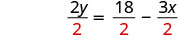
Simplify.		Simplify.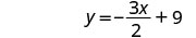

Try It 13

Solve the formula \(5x+2y=18\) for \(y\):

1. when \(x = 4\)
2. in general

Answer

1. \(y = -1\)
2. \(y = \frac{18 - 5x}{2}\)

Convert between Fahrenheit and Celsius Temperatures

Have you ever been in a foreign country and heard the weather forecast? If the forecast is for 22°C, what does that mean?

The U.S. and metric systems use different scales to measure temperature. The U.S. system uses degrees Fahrenheit, written °F. The metric system uses degrees Celsius, written °C. The figure below shows the relationship between the two systems.

TEMPERATURE CONVERSION

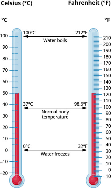
To convert from Fahrenheit temperature, F, to Celsius temperature, C, use the formula

\[C = \frac { 5 } { 9 } ( F - 32 )\nonumber\]

To convert from Celsius temperature, C, to Fahrenheit temperature, F, use the formula

\[F = \frac { 9 } { 5 } C + 32\nonumber\]

Example 14

Convert 50° Fahrenheit into degrees Celsius.

Solution

We will substitute 50°F into the formula to find C.

Simplify in parentheses.
Multiply.
	So we found that 50°F is equivalent to 10°C.

Try It 14

Convert the Fahrenheit temperature to degrees Celsius: 59° Fahrenheit.

Answer

15°C

Example 15

While visiting Paris, Woody noticed that the temperature was 20 °C. Convert the temperature into degrees Fahrenheit.

Solution

We will substitute 20°C into the formula to find F.

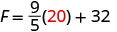Multiply.
Add.
	So we found that 20°C is equivalent to 68°F.

Try It 15

Convert the Celsius temperature to degrees Fahrenheit: The temperature in Helsinki, Finland, was 15 °C.

Answer

59°F