2.4: The Parabola

Last updated
Save as PDF

Page ID: 192241

$ \newcommand{\vecs}[1]{\overset { \scriptstyle \rightharpoonup} {\mathbf{#1}} } $

$ \newcommand{\vecd}[1]{\overset{-\!-\!\rightharpoonup}{\vphantom{a}\smash {#1}}} $

$ \newcommand{\dsum}{\displaystyle\sum\limits} $

$ \newcommand{\dint}{\displaystyle\int\limits} $

$ \newcommand{\dlim}{\displaystyle\lim\limits} $

$ \newcommand{\id}{\mathrm{id}}$ $ \newcommand{\Span}{\mathrm{span}}$

( \newcommand{\kernel}{\mathrm{null}\,}\) $ \newcommand{\range}{\mathrm{range}\,}$

$ \newcommand{\RealPart}{\mathrm{Re}}$ $ \newcommand{\ImaginaryPart}{\mathrm{Im}}$

$ \newcommand{\Argument}{\mathrm{Arg}}$ $ \newcommand{\norm}[1]{\| #1 \|}$

$ \newcommand{\inner}[2]{\langle #1, #2 \rangle}$

$ \newcommand{\Span}{\mathrm{span}}$

$ \newcommand{\id}{\mathrm{id}}$

$ \newcommand{\Span}{\mathrm{span}}$

$ \newcommand{\kernel}{\mathrm{null}\,}$

$ \newcommand{\range}{\mathrm{range}\,}$

$ \newcommand{\RealPart}{\mathrm{Re}}$

$ \newcommand{\ImaginaryPart}{\mathrm{Im}}$

$ \newcommand{\Argument}{\mathrm{Arg}}$

$ \newcommand{\norm}[1]{\| #1 \|}$

$ \newcommand{\inner}[2]{\langle #1, #2 \rangle}$

$ \newcommand{\Span}{\mathrm{span}}$ $ \newcommand{\AA}{\unicode[.8,0]{x212B}}$

$ \newcommand{\vectorA}[1]{\vec{#1}} % arrow$

$ \newcommand{\vectorAt}[1]{\vec{\text{#1}}} % arrow$

$ \newcommand{\vectorB}[1]{\overset { \scriptstyle \rightharpoonup} {\mathbf{#1}} } $

$ \newcommand{\vectorC}[1]{\textbf{#1}} $

$ \newcommand{\vectorD}[1]{\overrightarrow{#1}} $

$ \newcommand{\vectorDt}[1]{\overrightarrow{\text{#1}}} $

$ \newcommand{\vectE}[1]{\overset{-\!-\!\rightharpoonup}{\vphantom{a}\smash{\mathbf {#1}}}} $

$ \newcommand{\vecs}[1]{\overset { \scriptstyle \rightharpoonup} {\mathbf{#1}} } $

$\newcommand{\longvect}{\overrightarrow}$

$ \newcommand{\vecd}[1]{\overset{-\!-\!\rightharpoonup}{\vphantom{a}\smash {#1}}} $

$\newcommand{\avec}{\mathbf a}$ $\newcommand{\bvec}{\mathbf b}$ $\newcommand{\cvec}{\mathbf c}$ $\newcommand{\dvec}{\mathbf d}$ $\newcommand{\dtil}{\widetilde{\mathbf d}}$ $\newcommand{\evec}{\mathbf e}$ $\newcommand{\fvec}{\mathbf f}$ $\newcommand{\nvec}{\mathbf n}$ $\newcommand{\pvec}{\mathbf p}$ $\newcommand{\qvec}{\mathbf q}$ $\newcommand{\svec}{\mathbf s}$ $\newcommand{\tvec}{\mathbf t}$ $\newcommand{\uvec}{\mathbf u}$ $\newcommand{\vvec}{\mathbf v}$ $\newcommand{\wvec}{\mathbf w}$ $\newcommand{\xvec}{\mathbf x}$ $\newcommand{\yvec}{\mathbf y}$ $\newcommand{\zvec}{\mathbf z}$ $\newcommand{\rvec}{\mathbf r}$ $\newcommand{\mvec}{\mathbf m}$ $\newcommand{\zerovec}{\mathbf 0}$ $\newcommand{\onevec}{\mathbf 1}$ $\newcommand{\real}{\mathbb R}$ $\newcommand{\twovec}[2]{\left[\begin{array}{r}#1 \\ #2 \end{array}\right]}$ $\newcommand{\ctwovec}[2]{\left[\begin{array}{c}#1 \\ #2 \end{array}\right]}$ $\newcommand{\threevec}[3]{\left[\begin{array}{r}#1 \\ #2 \\ #3 \end{array}\right]}$ $\newcommand{\cthreevec}[3]{\left[\begin{array}{c}#1 \\ #2 \\ #3 \end{array}\right]}$ $\newcommand{\fourvec}[4]{\left[\begin{array}{r}#1 \\ #2 \\ #3 \\ #4 \end{array}\right]}$ $\newcommand{\cfourvec}[4]{\left[\begin{array}{c}#1 \\ #2 \\ #3 \\ #4 \end{array}\right]}$ $\newcommand{\fivevec}[5]{\left[\begin{array}{r}#1 \\ #2 \\ #3 \\ #4 \\ #5 \\ \end{array}\right]}$ $\newcommand{\cfivevec}[5]{\left[\begin{array}{c}#1 \\ #2 \\ #3 \\ #4 \\ #5 \\ \end{array}\right]}$ $\newcommand{\mattwo}[4]{\left[\begin{array}{rr}#1 \amp #2 \\ #3 \amp #4 \\ \end{array}\right]}$ $\newcommand{\laspan}[1]{\text{Span}\{#1\}}$ $\newcommand{\bcal}{\cal B}$ $\newcommand{\ccal}{\cal C}$ $\newcommand{\scal}{\cal S}$ $\newcommand{\wcal}{\cal W}$ $\newcommand{\ecal}{\cal E}$ $\newcommand{\coords}[2]{\left\{#1\right\}_{#2}}$ $\newcommand{\gray}[1]{\color{gray}{#1}}$ $\newcommand{\lgray}[1]{\color{lightgray}{#1}}$ $\newcommand{\rank}{\operatorname{rank}}$ $\newcommand{\row}{\text{Row}}$ $\newcommand{\col}{\text{Col}}$ $\renewcommand{\row}{\text{Row}}$ $\newcommand{\nul}{\text{Nul}}$ $\newcommand{\var}{\text{Var}}$ $\newcommand{\corr}{\text{corr}}$ $\newcommand{\len}[1]{\left|#1\right|}$ $\newcommand{\bbar}{\overline{\bvec}}$ $\newcommand{\bhat}{\widehat{\bvec}}$ $\newcommand{\bperp}{\bvec^\perp}$ $\newcommand{\xhat}{\widehat{\xvec}}$ $\newcommand{\vhat}{\widehat{\vvec}}$ $\newcommand{\uhat}{\widehat{\uvec}}$ $\newcommand{\what}{\widehat{\wvec}}$ $\newcommand{\Sighat}{\widehat{\Sigma}}$ $\newcommand{\lt}{<}$ $\newcommand{\gt}{>}$ $\newcommand{\amp}{&}$ $\definecolor{fillinmathshade}{gray}{0.9}$

Learning Objectives

Sketch a graph of the basic quadratic function $f(x)=x^2$
Use scaling, shifting, and reflecting to sketch the graph of the quadratic function $f(x)=a(x-h)^{2}+k$
Use the technique of completing the square to change a quadratic function from standard form to vertex form

In this section, you will learn how to draw the graph of the quadratic function defined by the equation

\[f(x)=a(x-h)^{2}+k \label{eq1}\nonumber \]

You will quickly learn that the graph of the quadratic function is shaped like a "U" and is called a parabola. This form of the quadratic function is called vertex form, so named because the form easily reveals the vertex or “turning point” of the parabola. Each of the constants in the vertex form of the quadratic function plays a role. As you will soon see, the constant $a$ controls the scaling (stretching or compressing of the parabola), the constant $h$ controls a horizontal shift and placement of the axis of symmetry, and the constant $k$ controls the vertical shift. Let’s begin by looking at the scaling of the quadratic.

Scaling the Quadratic

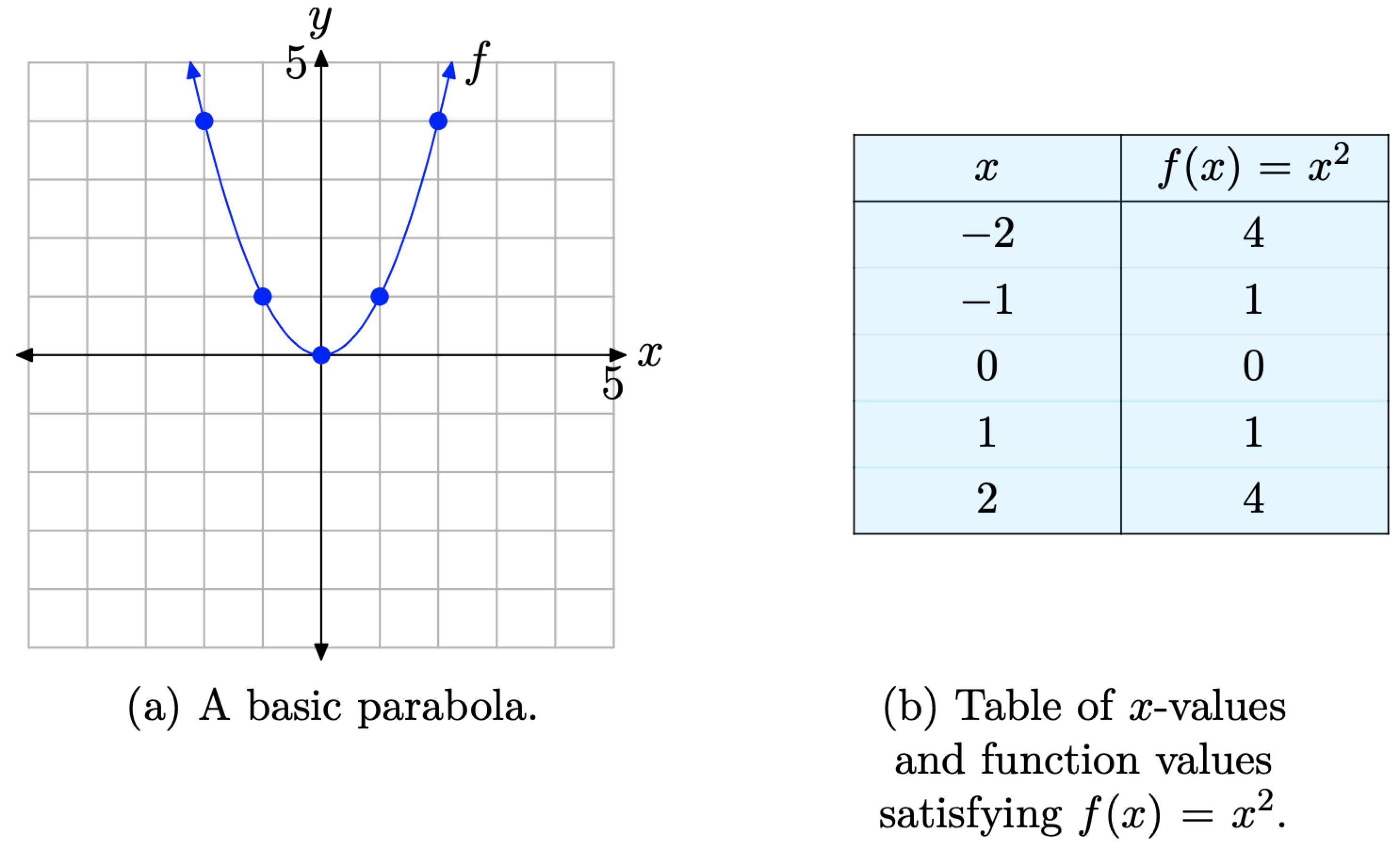
The graph of the basic quadratic function $f(x)=x^{2}$ shown below is a parabola. We say that the parabola in the figure below “opens upward.” The point at (0, 0), the “turning point” of the parabola, is called the vertex of the parabola. We’ve tabulated a few points for reference in the table and then superimposed these points on the graph of $f(x)=x^{2}$.

Now that we know the basic shape of the parabola determined by $f(x) = x^{2}$, let’s see what happens when we scale the graph of $f(x) = x^{2}$ in the vertical direction. For example, let’s investigate the graph of $g(x) = 2x^{2}$. The factor of 2 has a doubling effect. Note that each of the function values of g is twice the corresponding function value of $f$ in the table.

Stretching Factor

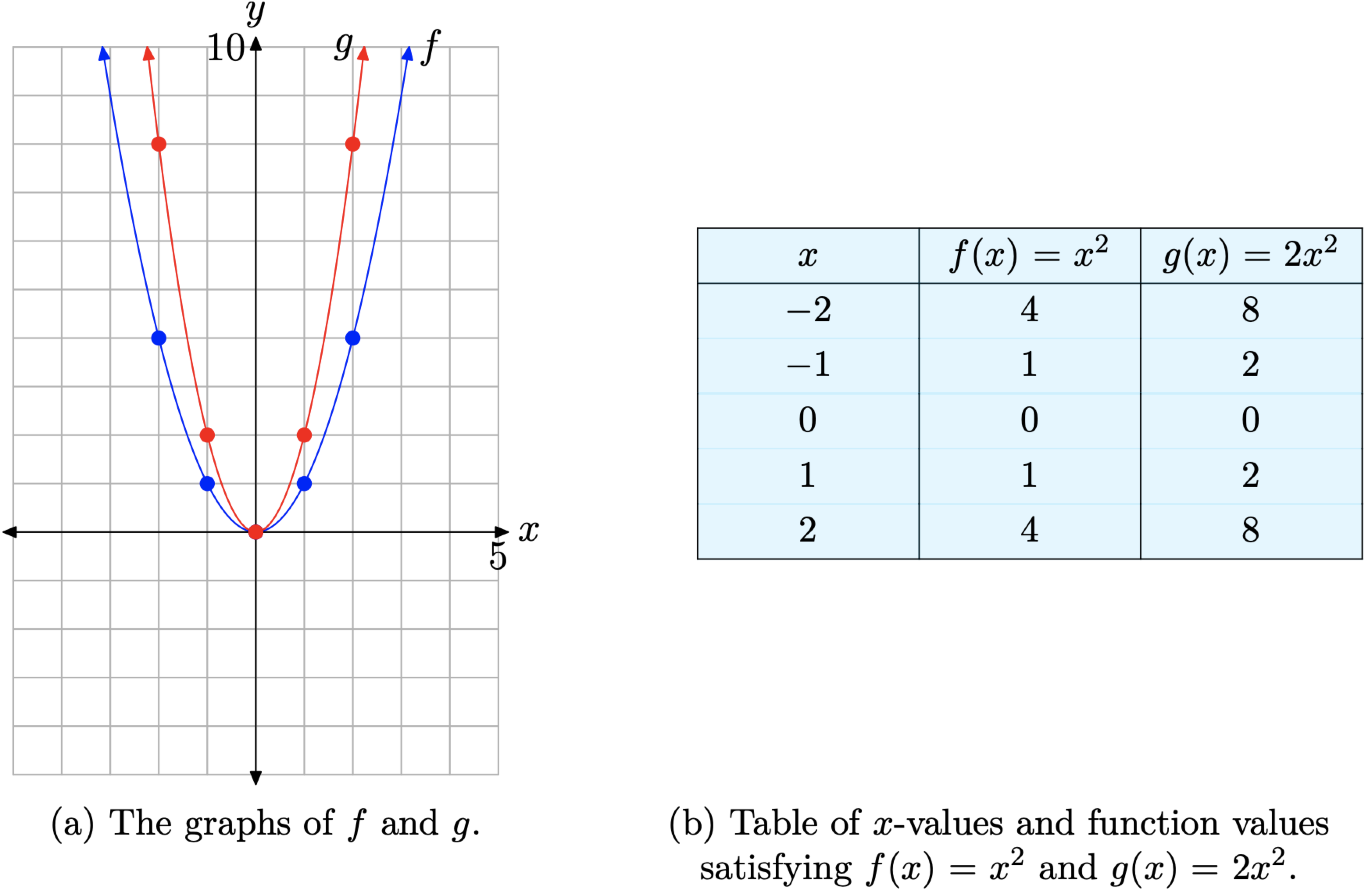
If a is a constant larger than 1, that is, if $a > 1$, then the graph of $g(x) = ax^{2}$, when compared with the graph of $f(x) = x^{2}$, is stretched by a factor of $a$.

Next, let’s consider what happens when we scale by a number that is smaller than 1 (but greater than zero — we’ll deal with the negative in a moment). For example, let’s investigate the graph of $g(x) = (1/2)x^{2}$. The factor 1/2 has a halving effect. Note that each of the function values of g is half the corresponding function value of f in the table below.

Compression Factor

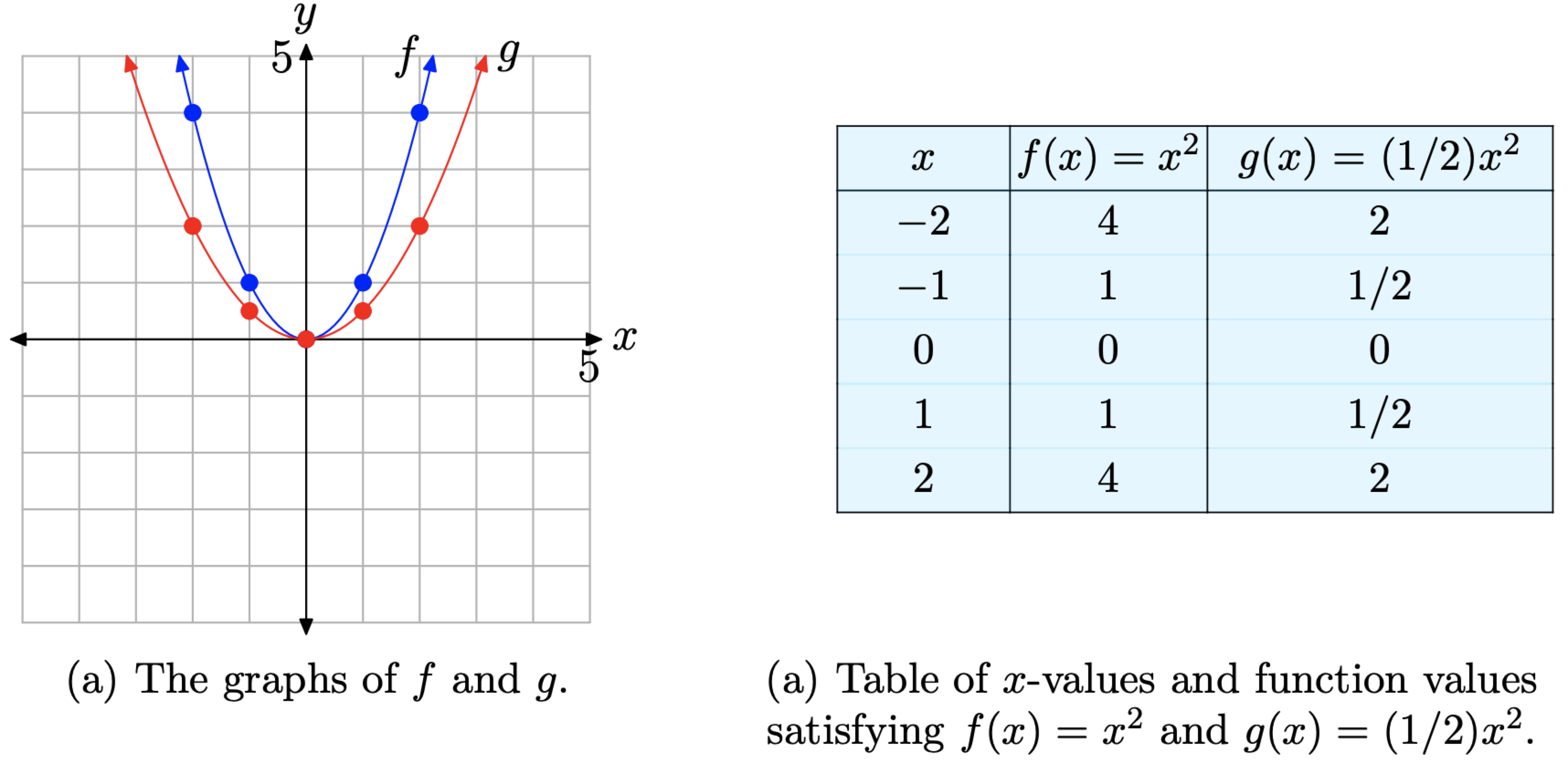
If a is a constant smaller than 1 (but larger than zero), that is, if $0 < a < 1$, then the graph of $g(x) = ax^{2}$, when compared with the graph of $f(x) = x^{2}$, is compressed by a factor of $\dfrac{1}{a}$.

Some find this somewhat counterintuitive. However, if you compare the function $g(x) = (1/2)x^2$ with the general form $g(x) = ax^2$, you see that $a=\dfrac{1}{2}$. This property states that the graph will be compressed by a factor of $\dfrac{1}{a}$. In this case, $a=1/2$ and

\[\frac{1}{a}=\frac{1}{1 / 2}=2 \nonumber \]

Thus, the graph of $g(x) = (1/2)x^2$ should be compressed by a factor of 1/(1/2) or 2.

Vertical Reflections

Let’s consider the graph of $g(x) = ax^2$, when a < 0. For example, consider the graphs of $g(x)=-x^{2}$ and $h(x)=(-1 / 2) x^{2}$ shown here.

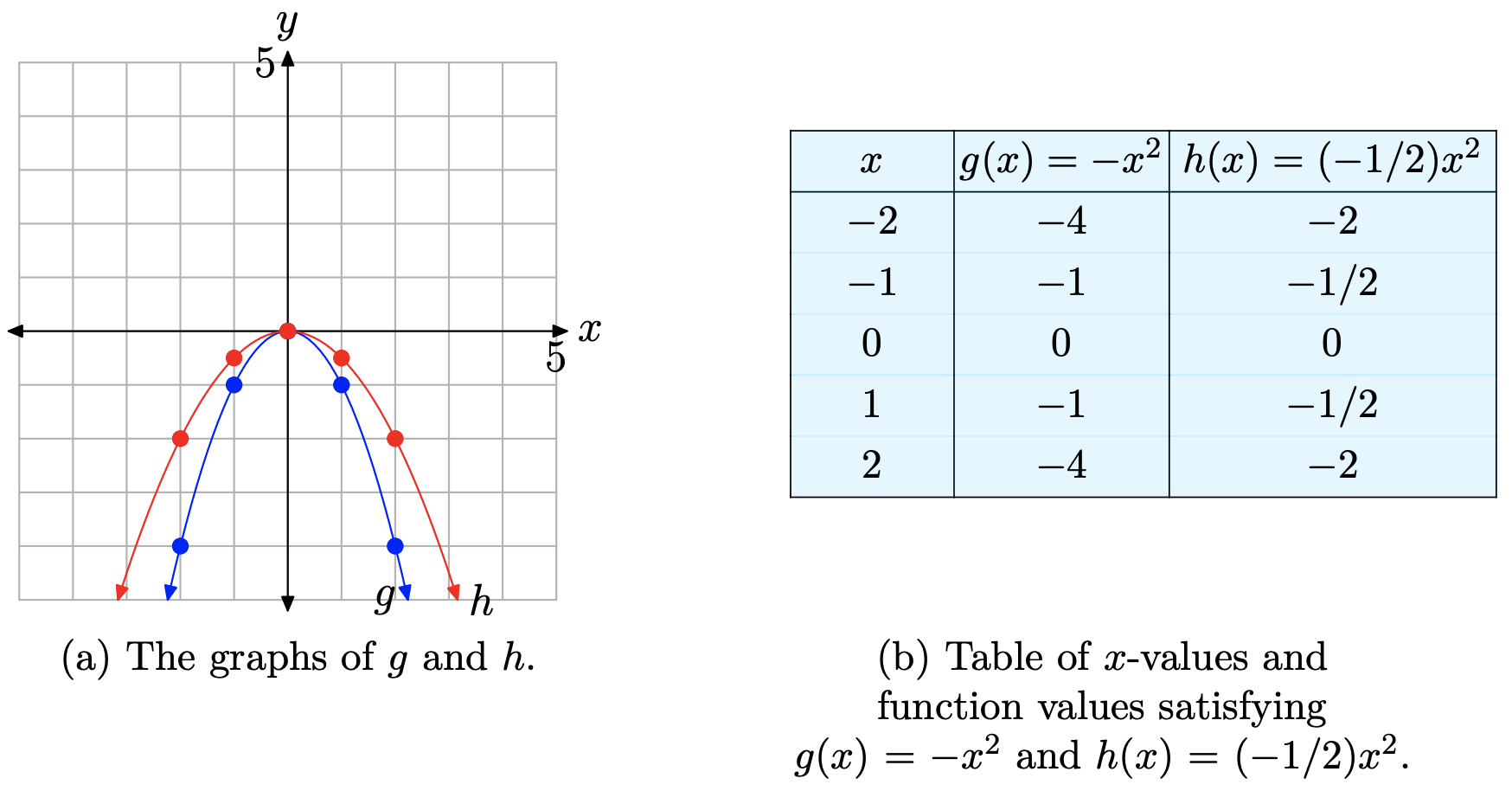
When the two tables are compared, it is easy to see that the numbers in the last two columns are the same, but they’ve been negated. The graphs have been reflected across the $x$-axis. Each of the parabolas now “opens downward.”

However, it is encouraging to see that the scaling role of the constant a in $g(x) = ax^2$ remains unchanged. In the case of $h(x) = (−1/2)x^2$, the $y$-values are still “compressed” by a factor of two, but the minus sign negates these values, causing the graph to reflect across the $x$-axis. Thus, for example, one would think that the graph of $y = −2x^2$ would be stretched by a factor of two, then reflected across the $x$-axis. Indeed, this is correct, and this discussion leads to the following property.

Reflection Across $x$-axis

If $−1 < a < 0$, then the graph of $g(x) = ax^2$, when compared with the graph of $f(x) = x^2$, is compressed by a factor of 1/|a|, then reflected across the $x$-axis. Secondly, if a < −1, then the graph of $g(x) = ax^2$, when compared with the graph of $f(x) = x^2$, is stretched by a factor of |a|, then reflected across the $x$-axis.

Again, some find this Property confusing. However, if you compare $g(x) = (−1/2)x^2$ with the general form $g(x) = ax^2$, you see that a = −1/2. Note that in this case, −1 < a < 0. The property states that the graph will be compressed by a factor of 1/|a|. In this case, a = −1/2 and

\[\frac{1}{|a|}=\frac{1}{|-1 / 2|}=2 \nonumber \]

That is, the property states that the graph of $g(x) = (−1/2)x^2$ is compressed by a factor of 1/(| − 1/2|), or 2, then reflected across the $x$-axis. Note again that the vertex at the origin is unaffected by this scaling and reflection.

Horizontal Translations

The graph of $g(x) = (x + 1)^2$ below shows a basic parabola that is shifted one unit to the left. Examine the table and note that the equation $g(x) = (x + 1)^2$ produces the same $y$-values as does the equation $f(x) = x^2$, the only difference being that these $y$-values are calculated at $x$-values that are one unit less than those used for $f(x) = x^2$. Consequently, the graph of $g(x) = (x + 1)^2$ must shift one unit to the left of the graph of $f(x) = x^2$.

Note that this result is counterintuitive. One would think that replacing x with x + 1 would shift the graph one unit to the right, but the shift actually occurs in the opposite direction.

Finally, note that this time the vertex of the parabola has shifted 1 unit to the left and is now located at the point (−1, 0).

We are led to the following conclusion.

Shift to Left or Right

If c > 0, then the graph of $g(x) = (x + c)^2$ is shifted c units to the left of the graph of $f(x) = x^2$. However, if c > 0, then the graph of $g(x) = (x − c)^2$ is shifted c units to the right of the graph of $f(x) = x^2$.

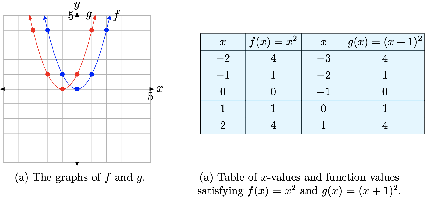
A similar thing happens when you replace x with x − 1, only this time the graph is shifted one unit to the right.

Vertical Translations

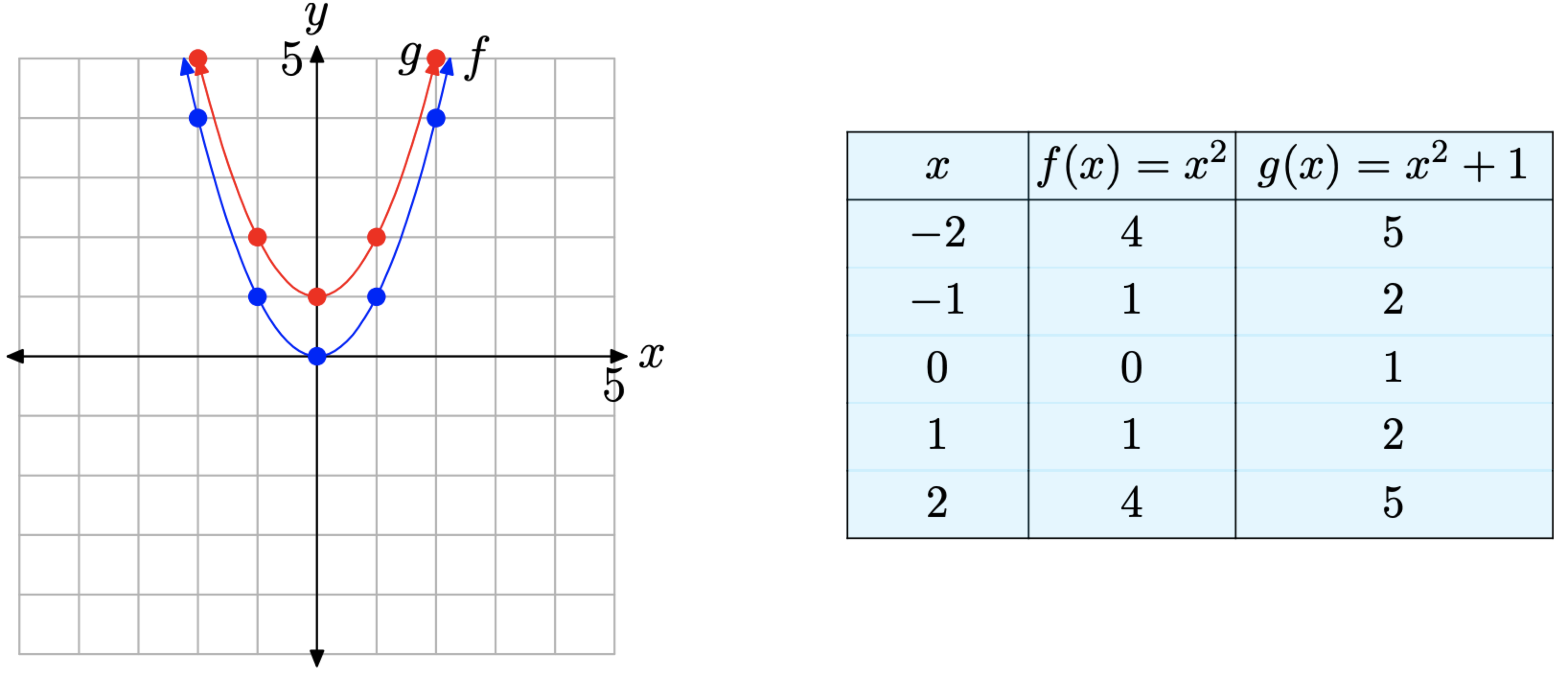
The graph of $g(x) = x^2 + 1$ is shifted one unit upward from the graph of $f(x) = x^2$. This is easy to see as both equations use the same $x$-values in the table, but the function values of $g(x) = x^2 + 1$ are one unit larger than the corresponding function values of $f(x) = x^2$.

Note that the vertex of the graph of $g(x) = x^2 + 1$ has also shifted upward 1 unit and is now located at the point (0, 1).

The above discussion leads to the following property.

Shift Up or Down

If c > 0, the graph of $g(x) = x^2 + c$ is shifted c units upward from the graph of $f(x) = x^2$. However, if c > 0, the graph of $g(x) = x^2 − c$ is shifted c units downward from the graph of $f(x) = x^2$.

In a similar vein, the graph of $y = x^2 − 1$ is shifted downward one unit from the graph of $y = x^2$.

The Axis of Symmetry

In the first figure we encountered, the graph of $y = x^2$ was symmetric with respect to the $y$-axis. One half of the parabola is a mirror image of the other with respect to the $y$-axis. We say the $y$-axis is acting as the axis of symmetry.

If the parabola is reflected across the $x$-axis, as in Figure 6, the axis of symmetry doesn’t change. The graph is still symmetric with respect to the $y$-axis. Similar comments apply to scalings and vertical translations. However, if the graph of $y = x^2$ is shifted right or left, then the axis of symmetry will change.

Example 1

Sketch the graph of $y = −(x + 2)^2 + 3$.

Solution

Although not required, this example is much simpler if you perform reflections before translations.

If at all possible, perform scalings and reflections before translations.

In the series shown in the next figure, we first perform a reflection, then a horizontal translation, followed by a vertical translation.

The graph of $y = −x^2$ is a reflection of the graph of $y = x^2$ across the $x$-axis and opens downward. Note that the vertex is still at the origin.
We’ve replaced x with x+ 2 in the equation $y = −x^2$ to obtain the equation $y = −(x+ 2)^2$. The effect is to shift the graph of $y = −x^2$ two units to the left to obtain the graph of $y = −(x+ 2)^2$. Note that the vertex is now at the point (−2, 0).
We’ve added 3 to the equation $y = −(x+ 2)^2$ to obtain the equation $y = −(x+ 2)^2 + 3$. The effect is to shift the graph of $y = −(x+ 2)2$ upward 3 units to obtain the graph of $y=-(x+2)^{2}+3$. Note that the vertex is now at the point (−2, 3).

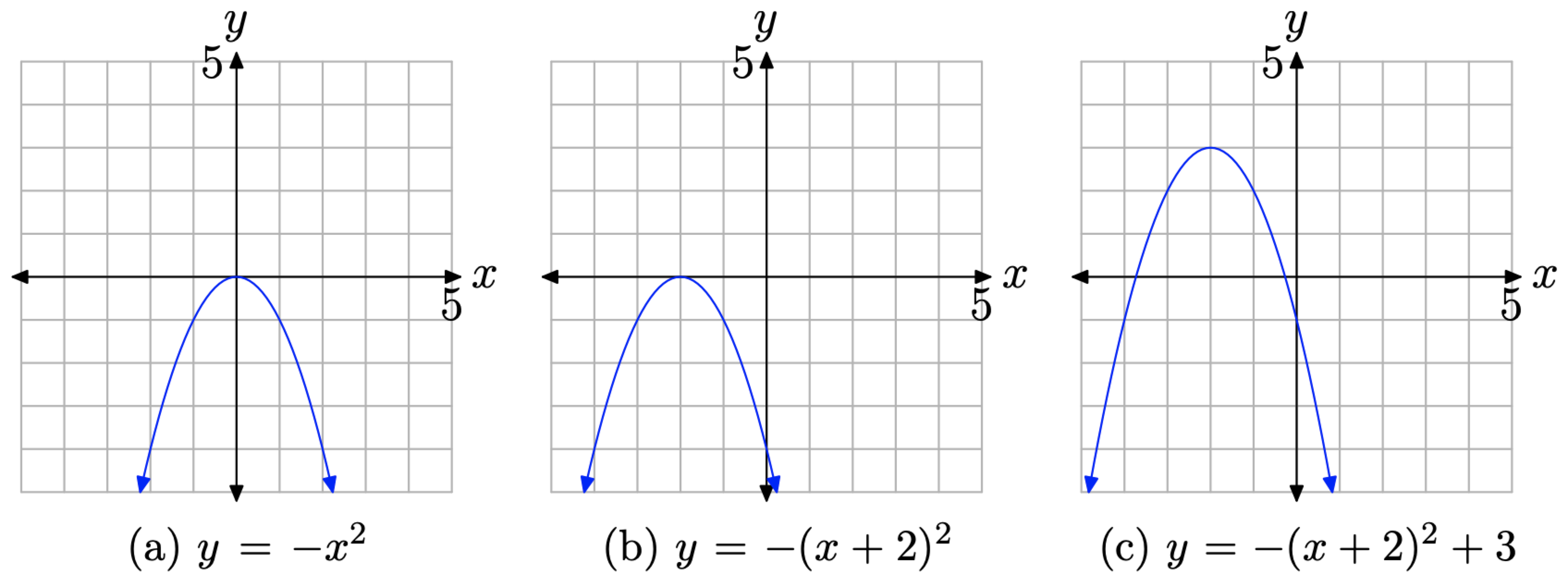
In practice, we can proceed more quickly. Analyze the equation $y=-(x+2)^{2}+3$. The minus sign indicates that the parabola opens downward. The presence of x + 2 indicates a shift of 2 units to the left. Finally, adding the 3 will shift the graph upward 3 units. Thus, we have a parabola that “opens downward” with a vertex at (−2, 3).

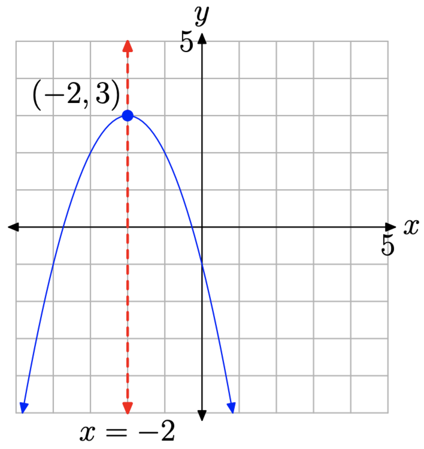
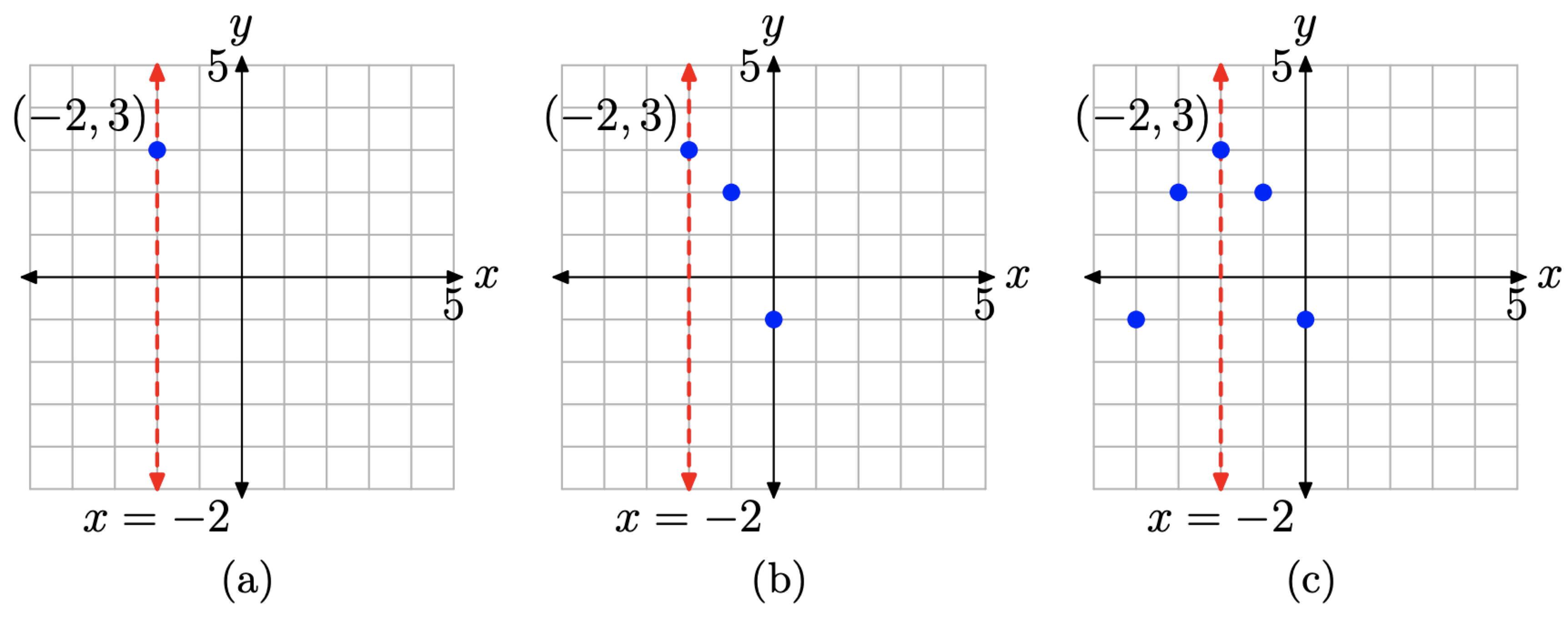
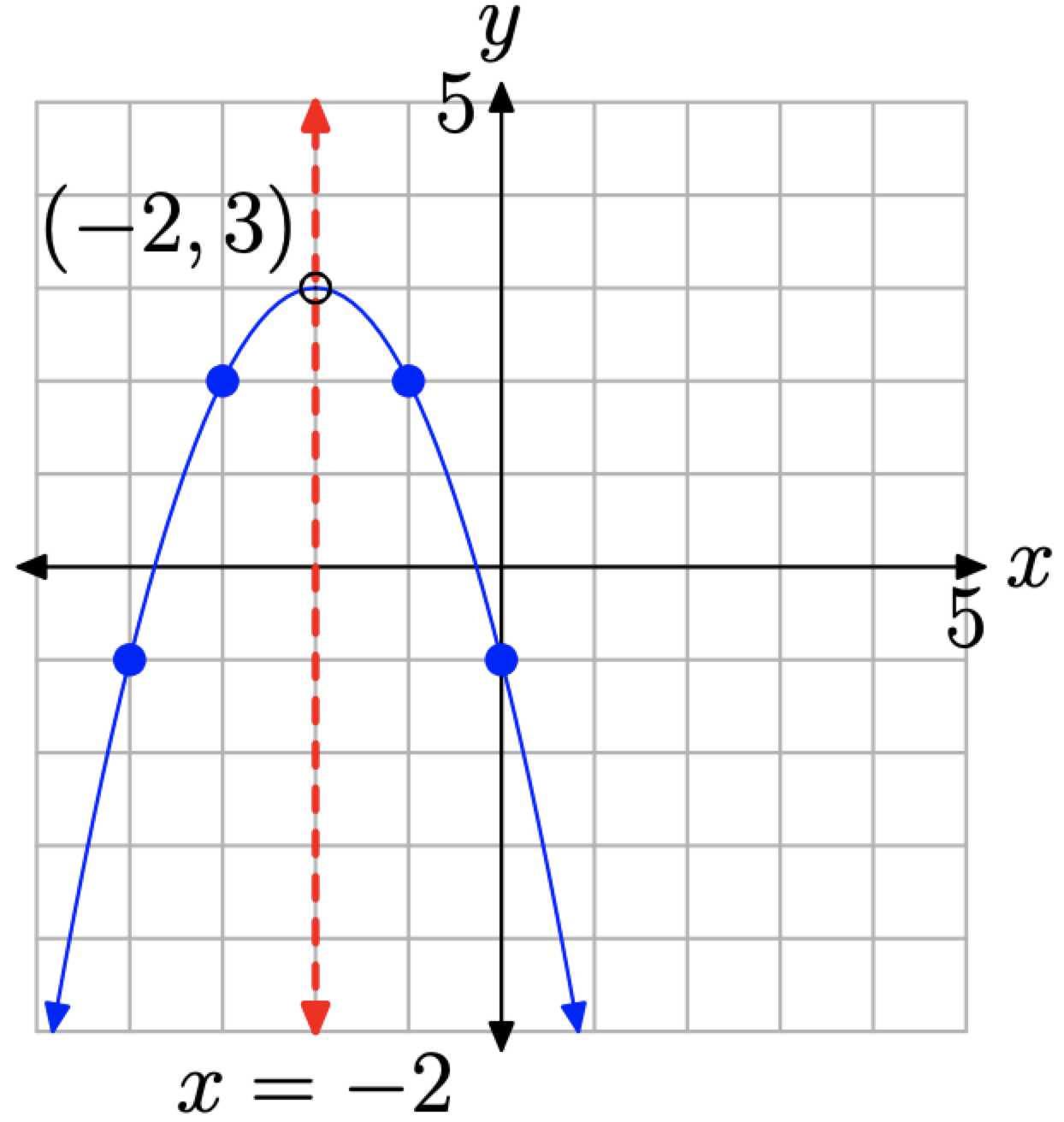
The axis of symmetry passes through the vertex (−2, 3) and has equation $x=−2$. Note that the right half of the parabola is a mirror image of its left half across this axis of symmetry. We can use the axis of symmetry to gain an accurate plot of the parabola with minimal plotting of points.

Guidelines for Using the Axis of Symmetry

Start by plotting the vertex and axis of symmetry.
Next, compute two points on either side of the axis of symmetry. We choose x = −1 and x = 0 and compute the corresponding $y$-values using the equation $y=-(x+2)^{2}+3$

x	$y=-(x+2)^{2}+3$
-1	2
0	-1

Plot the points from the table.
Finally, plot the mirror images of these points across the axis of symmetry, as shown in the figure.

$WeChat48fdea7a2bfc12a66715309981d3043d.png$

The image in the far right graph clearly contains enough information to complete the graph of the parabola having equation $y=-(x+2)^{2}+3$.

Let’s summarize what we’ve seen thus far.

Summary

The form of the quadratic function \[f(x)=a(x-h)^{2}+k \nonumber \] is called vertex form. The graph of this quadratic function is a parabola.

The graph of the parabola opens upward if a > 0, downward if a < 0.
If the magnitude of a is larger than 1, then the graph of the parabola is stretched by a factor of a. If the magnitude of a is smaller than 1, then the graph of the parabola is compressed by a factor of 1/a.
The parabola is translated h units to the right if h > 0, and h units to the left if h < 0.
The parabola is translated k units upward if k > 0, and k units downward if k < 0.
The coordinates of the vertex are (h, k).
The axis of symmetry is a vertical line through the vertex whose equation is x = h.

Complete The Square

So far, you learned that it is a simple task to sketch the graph of a quadratic function if it is presented in vertex form

\[f(x)=a(x-h)^{2}+k \nonumber \]

The goal of the current section is to start with the most general form of the quadratic function, namely

\[f(x)=a x^{2}+b x+c \nonumber \]

and manipulate the equation into vertex form. Once you have your quadratic function in vertex form, the technique of the previous section should allow you to construct the graph of the quadratic function.

We will use special product formulas for perfect square trinomials:

\[(a+b)^2=a^2+2ab+b^2\quad\text{or}\quad (a-b)^2=a^2-2ab+b^2\nonumber\]

We use these formulas to help us solve by completing the square.

We first begin by completing the square and rewriting the trinomial in factored form using the perfect square trinomial formulas.

Example 2

Complete the square by finding $c$: $x^2+8x+c$

Solution

There are several ways to complete the square. The first way is to mentally think about a number for $c$ such that we can factor the trinomial as a perfect square trinomial, i.e.,

\[x^2+8x+c=(x+\underline{\quad} )^2\nonumber\]

Some might see that this number $c = 16$ if they are keen at factoring. Notice, $(x + 4)^2 = x^2 + 8x + 16$. Another way is to, literally, complete the square:

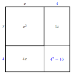
Notice the square has all components of the perfect square trinomial. Hence, we can see the dimensions of this square to be

\[(x+4)\times (x+4)\nonumber\]

which is

\[(x+4)^2\nonumber\]

and the missing constant coefficient is $16$, the square of $4$. Using one of these methods will suffice, depending on the learner. Some students enjoy the geometric relationship between the quadratic equation and the square, and some enjoy the algebraic method. It is up to the discretion of the student.

Thus, we see $c = 16$ and the perfect square trinomial $x^2 + 8x + \color{blue}{16}$ is factored into $(x + 4)^2$.

Note

To complete the square of any trinomial, we always square half of the linear term’s coefficient, i.e.,

\[\left(\dfrac{b}{2}\right)^2\quad\text{or}\quad\left(\dfrac{1}{2}b\right)^2\nonumber\]

We usually use the second expression when the middle term's coefficient is a fraction.

Example 3

Complete the square by finding $c$: $x^2-7x+c$

Solution

To obtain $c$, we use the formula above $\left(\dfrac{b}{2}\right)^2$.

\[\begin{array}{rl} x^2-7x+\color{blue}{c}&\color{black}{b}=-7;\text{ apply formula }\left(\dfrac{b}{2}\right)^2 \\ x^2-7x+\color{blue}{\left(\dfrac{-7}{2}\right)^2}&\color{black}{\text{Simplify }}c\\ x^2-7x+\color{blue}{\dfrac{49}{4}}&\color{black}{\text{Perfect square trinomial}}\end{array}\nonumber\]

Thus, $c=\dfrac{49}{4}$. Rewriting this perfect square trinomial in factored form, we get

\[x^2-7x+\color{blue}{\dfrac{49}{4}}\color{black}{=}\left(x-\dfrac{7}{2}\right)^2\nonumber\]

Working with $f(x) = x^2 + bx + c$

The examples in this section will have the form $f(x) = x^2 + bx + c$. Note that the coefficient of $x^2$ is 1. In the next section, we will work with a harder form, $f(x) = ax^2 + bx + c$, where $a \neq 1$.

Algorithm for Completing the Square

The procedure for completing the square involves three key steps.

Take half of the coefficient of x and square the result.
Add and subtract the quantity from step one so that the right-hand side of the equation does not change.
Factor the resulting perfect square trinomial and combine constant terms.

Let’s follow this procedure and place $f(x) = x^2 + 4x + 7$ in vertex form.

Take half of the coefficient of x. Thus, (1/2)(4) = 2. Square this result. Thus, $2^2 = 4$.
Add and subtract 4 on the right side of the equation $f(x) = x^2 + 4x + 7$ \[f(x)=x^{2}+4 x+4-4+7 \nonumber \]
Group the first three terms on the right-hand side. These form a perfect square trinomial.

\[f(x)=\left(x^{2}+4 x+4\right)-4+7 \nonumber \]

Now factor the perfect square trinomial and combine the constants at the end to get

\[f(x)=(x+2)^{2}+3 \nonumber \]

That’s it, we’re done! We’ve returned the general quadratic $f(x) = x^2 + 4x + 7$ back to vertex form $f(x) = (x + 2)^2 + 3$.

Example 4

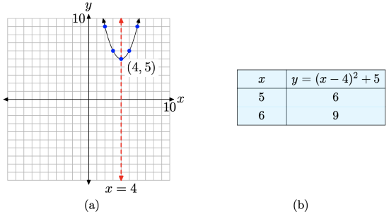
Complete the square to place $f(x) = x^2 − 8x + 21$ in vertex form and sketch its graph.

Solution

First, take half of the coefficient of x and square; i.e., $[(1/2)(−8)]^2 = 16$. On the right side of the equation, add and subtract this amount so as to not change the equation.

\[f(x)=x^{2}-8 x+16-16+21 \nonumber \]

Group the first three terms on the right-hand side of the equation.

\[f(x)=\left(x^{2}-8 x+16\right)-16+21 \nonumber \]

The first three terms form a perfect square trinomial that is easily factored. Also, combine constants at the end.

\[f(x)=(x-4)^{2}+5 \nonumber \]

This is a parabola that opens upward. We need to shift the parabola 4 units to the right and then 5 units upward, placing the vertex at (4, 5). The table calculates two points to the right of the axis of symmetry, and mirror points on the left of the axis of symmetry make for an accurate plot of the parabola.

Working with $f(x) = ax^2 + bx + c$

In the last two examples, the coefficient of $x^2$ was 1. In this section, we will learn how to complete the square when the coefficient of $x^2$ is some number other than 1.

Example 5

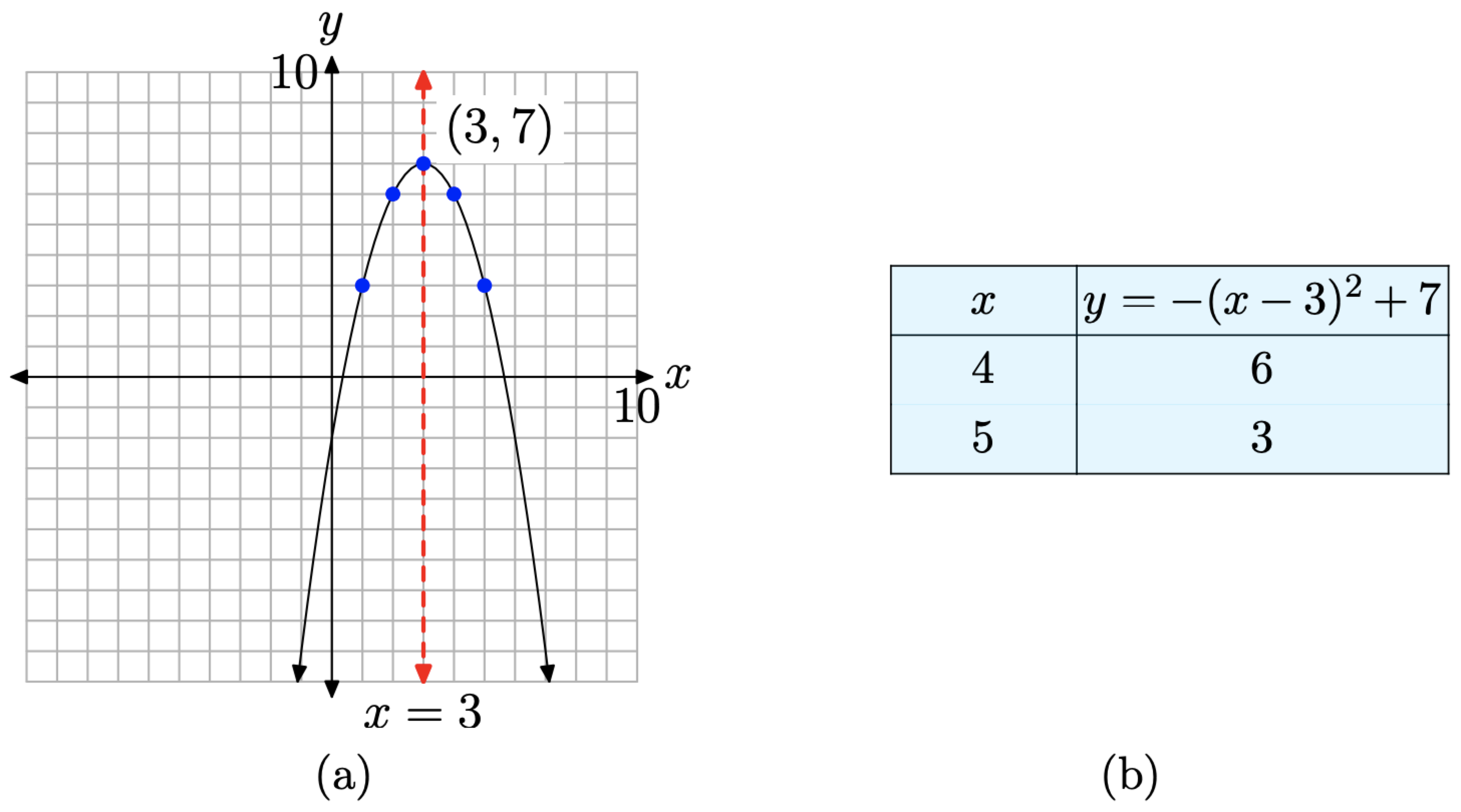
Complete the square to place $f(x) = −x^2 + 6x − 2$ in vertex form and sketch its graph.

Solution

If we factor out the coefficient of $x^2$, this will leave us with a trinomial having a leading coefficient of 1, which enables us to proceed much as we did before: halve the middle coefficient and square, add and subtract this amount, and factor the resulting perfect square trinomial. Since we were successful with this technique in the last example, let’s begin by factoring out the leading coefficient, in this case −1.

\[f(x)=-1\left[x^{2}-6 x+2\right] \nonumber \]

If we ignore the factor of −1 out front, the coefficient of $x^2$ in the trinomial expression inside the parentheses is a 1. Again, familiar ground! We will proceed as we did before, but we will carry the factor of −1 outside the parentheses in each step. Start by taking half of the coefficient of x and squaring the result; i.e., $[(1/2)(−6)]^2 = 9$.

Add and subtract this amount inside the parentheses so as to not change the equation.

\[f(x)=-1\left[x^{2}-6 x+9-9+2\right] \nonumber \]

Group the first three terms inside the parentheses and combine constants.

\[f(x)=-1\left[\left(x^{2}-6 x+9\right)-7\right] \nonumber \]

The grouped terms inside the parentheses form a perfect square trinomial that is easily factored.

\[f(x)=-1\left[(x-3)^{2}-7\right] \nonumber \]

Finally, redistribute the −1.

\[f(x)=-(x-3)^{2}+7 \nonumber \]

This is a parabola that opens downward. The parabola is also shifted 3 units to the right, then 7 units upward, placing the vertex at (3, 7). The table calculates two points to the right of the axis of symmetry, and mirror points on the left of the axis of symmetry make for an accurate plot of the parabola.

Let’s try one more example.

Example 6

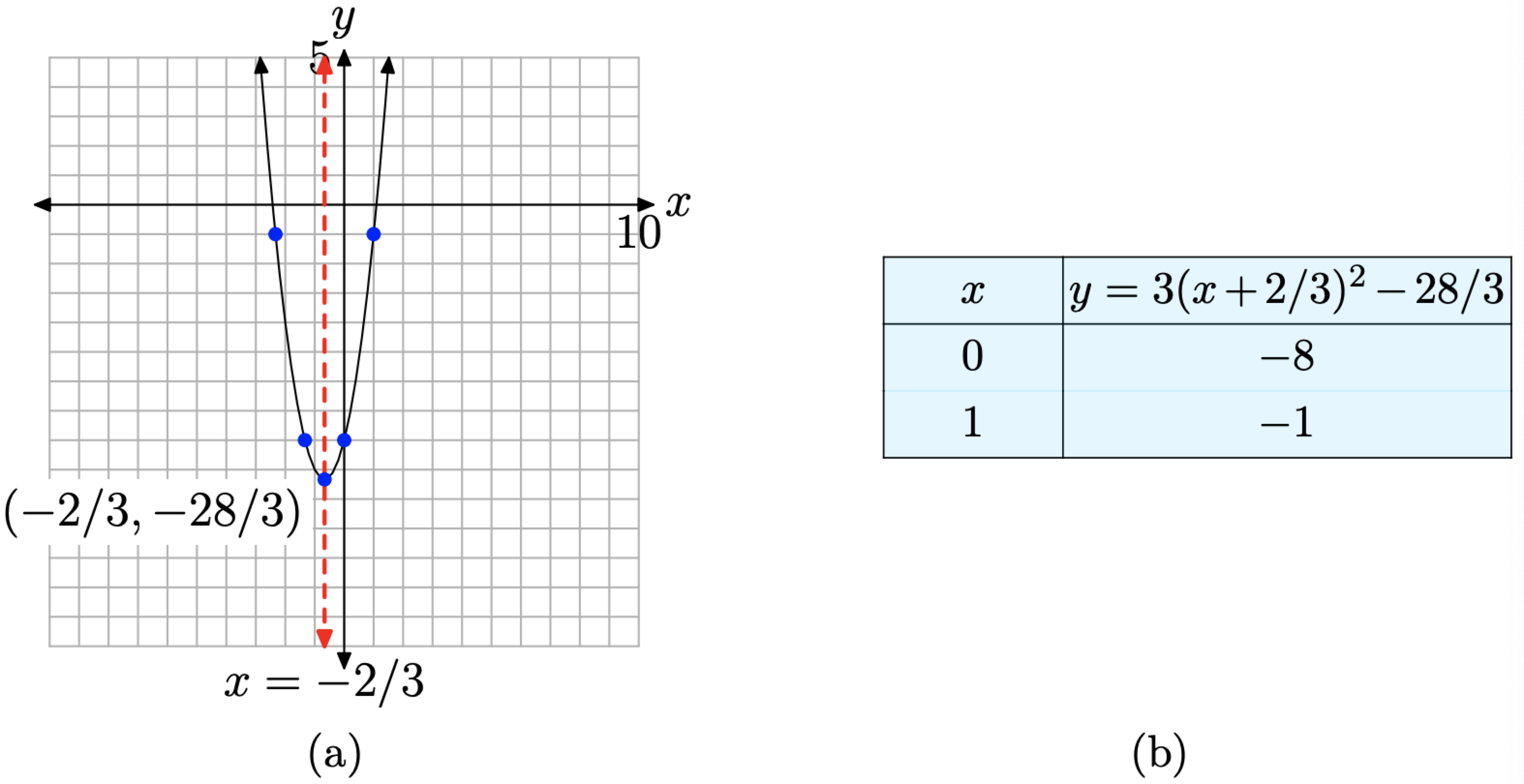
Complete the square to place $f(x) = 3x^2 + 4x − 8$ in vertex form and sketch its graph.

Solution

Let’s begin again by factoring out the leading coefficient, in this case a 3.

\[f(x)=3\left[x^{2}+\frac{4}{3} x-\frac{8}{3}\right] \nonumber \]

Fractions add a degree of difficulty, but, if you follow the same routine as in the previous examples, you should be able to get the needed result. Take half of the coefficient of x and square the result; i.e., $[(1/2)(4/3)]^2 = [2/3]^2 = 4/9$.

Add and subtract this amount inside the parentheses so as to not change the equation.

\[f(x)=3\left[x^{2}+\frac{4}{3} x+\frac{4}{9}-\frac{4}{9}-\frac{8}{3}\right] \nonumber \]

Group the first three terms inside the parentheses. You’ll need a common denominator to combine constants.

\[f(x)=3\left[\left(x^{2}+\frac{4}{3} x+\frac{4}{9}\right)-\frac{4}{9}-\frac{24}{9}\right] \nonumber \]

The grouped terms inside the parentheses form a perfect square trinomial that is easily factored.

\[f(x)=3\left[\left(x+\frac{2}{3}\right)^{2}-\frac{28}{9}\right] \nonumber \]

Finally, redistribute the 3.

\[f(x)=3\left(x+\frac{2}{3}\right)^{2}-\frac{28}{3} \nonumber \]

This is a parabola that opens upward. It is also stretched by a factor of 3, so it will be narrower than all of our previous examples. The parabola is also shifted 2/3 units to the left, then 28/3 units downward, placing the vertex at (−2/3, −28/3). The table calculates two points to the right of the axis of symmetry, and mirror points on the left of the axis of symmetry make for an accurate plot of the parabola.

$WeChat011edb36558dd8ef5de6a7bb305f3642.png$