4.1: An Introduction to The Graphs of Polynomial Functions

Last updated

Aug 1, 2025
Save as PDF
- 4: Polynomial and Rational Functions.
- 4.1E: Power Functions (Exercises)

Jason Gardner
The OpenTextBookStore

$\newcommand{\vecs}[1]{\overset { \scriptstyle \rightharpoonup} {\mathbf{#1}} }$

$\newcommand{\vecd}[1]{\overset{-\!-\!\rightharpoonup}{\vphantom{a}\smash {#1}}}$

$\newcommand{\id}{\mathrm{id}}$ $\newcommand{\Span}{\mathrm{span}}$

( \newcommand{\kernel}{\mathrm{null}\,}\) $\newcommand{\range}{\mathrm{range}\,}$

$\newcommand{\RealPart}{\mathrm{Re}}$ $\newcommand{\ImaginaryPart}{\mathrm{Im}}$

$\newcommand{\Argument}{\mathrm{Arg}}$ $\newcommand{\norm}[1]{\| #1 \|}$

$\newcommand{\inner}[2]{\langle #1, #2 \rangle}$

$\newcommand{\Span}{\mathrm{span}}$

$\newcommand{\id}{\mathrm{id}}$

$\newcommand{\Span}{\mathrm{span}}$

$\newcommand{\kernel}{\mathrm{null}\,}$

$\newcommand{\range}{\mathrm{range}\,}$

$\newcommand{\RealPart}{\mathrm{Re}}$

$\newcommand{\ImaginaryPart}{\mathrm{Im}}$

$\newcommand{\Argument}{\mathrm{Arg}}$

$\newcommand{\norm}[1]{\| #1 \|}$

$\newcommand{\inner}[2]{\langle #1, #2 \rangle}$

$\newcommand{\Span}{\mathrm{span}}$ $\newcommand{\AA}{\unicode[.8,0]{x212B}}$

$\newcommand{\vectorA}[1]{\vec{#1}} % arrow$

$\newcommand{\vectorAt}[1]{\vec{\text{#1}}} % arrow$

$\newcommand{\vectorB}[1]{\overset { \scriptstyle \rightharpoonup} {\mathbf{#1}} }$

$\newcommand{\vectorC}[1]{\textbf{#1}}$

$\newcommand{\vectorD}[1]{\overrightarrow{#1}}$

$\newcommand{\vectorDt}[1]{\overrightarrow{\text{#1}}}$

$\newcommand{\vectE}[1]{\overset{-\!-\!\rightharpoonup}{\vphantom{a}\smash{\mathbf {#1}}}}$

$\newcommand{\vecs}[1]{\overset { \scriptstyle \rightharpoonup} {\mathbf{#1}} }$

$\newcommand{\vecd}[1]{\overset{-\!-\!\rightharpoonup}{\vphantom{a}\smash {#1}}}$

$\newcommand{\avec}{\mathbf a}$

$\newcommand{\bvec}{\mathbf b}$

$\newcommand{\cvec}{\mathbf c}$

$\newcommand{\dvec}{\mathbf d}$

$\newcommand{\dtil}{\widetilde{\mathbf d}}$

$\newcommand{\evec}{\mathbf e}$

$\newcommand{\fvec}{\mathbf f}$

$\newcommand{\nvec}{\mathbf n}$

$\newcommand{\pvec}{\mathbf p}$

$\newcommand{\qvec}{\mathbf q}$

$\newcommand{\svec}{\mathbf s}$

$\newcommand{\tvec}{\mathbf t}$

$\newcommand{\uvec}{\mathbf u}$

$\newcommand{\vvec}{\mathbf v}$

$\newcommand{\wvec}{\mathbf w}$

$\newcommand{\xvec}{\mathbf x}$

$\newcommand{\yvec}{\mathbf y}$

$\newcommand{\zvec}{\mathbf z}$

$\newcommand{\rvec}{\mathbf r}$

$\newcommand{\mvec}{\mathbf m}$

$\newcommand{\zerovec}{\mathbf 0}$

$\newcommand{\onevec}{\mathbf 1}$

$\newcommand{\real}{\mathbb R}$

$\newcommand{\twovec}[2]{\left[\begin{array}{r}#1 \\ #2 \end{array}\right]}$

$\newcommand{\ctwovec}[2]{\left[\begin{array}{c}#1 \\ #2 \end{array}\right]}$

$\newcommand{\threevec}[3]{\left[\begin{array}{r}#1 \\ #2 \\ #3 \end{array}\right]}$

$\newcommand{\cthreevec}[3]{\left[\begin{array}{c}#1 \\ #2 \\ #3 \end{array}\right]}$

$\newcommand{\fourvec}[4]{\left[\begin{array}{r}#1 \\ #2 \\ #3 \\ #4 \end{array}\right]}$

$\newcommand{\cfourvec}[4]{\left[\begin{array}{c}#1 \\ #2 \\ #3 \\ #4 \end{array}\right]}$

$\newcommand{\fivevec}[5]{\left[\begin{array}{r}#1 \\ #2 \\ #3 \\ #4 \\ #5 \\ \end{array}\right]}$

$\newcommand{\cfivevec}[5]{\left[\begin{array}{c}#1 \\ #2 \\ #3 \\ #4 \\ #5 \\ \end{array}\right]}$

$\newcommand{\mattwo}[4]{\left[\begin{array}{rr}#1 \amp #2 \\ #3 \amp #4 \\ \end{array}\right]}$

$\newcommand{\laspan}[1]{\text{Span}\{#1\}}$

$\newcommand{\bcal}{\cal B}$

$\newcommand{\ccal}{\cal C}$

$\newcommand{\scal}{\cal S}$

$\newcommand{\wcal}{\cal W}$

$\newcommand{\ecal}{\cal E}$

$\newcommand{\coords}[2]{\left\{#1\right\}_{#2}}$

$\newcommand{\gray}[1]{\color{gray}{#1}}$

$\newcommand{\lgray}[1]{\color{lightgray}{#1}}$

$\newcommand{\rank}{\operatorname{rank}}$

$\newcommand{\row}{\text{Row}}$

$\newcommand{\col}{\text{Col}}$

$\renewcommand{\row}{\text{Row}}$

$\newcommand{\nul}{\text{Nul}}$

$\newcommand{\var}{\text{Var}}$

$\newcommand{\corr}{\text{corr}}$

$\newcommand{\len}[1]{\left|#1\right|}$

$\newcommand{\bbar}{\overline{\bvec}}$

$\newcommand{\bhat}{\widehat{\bvec}}$

$\newcommand{\bperp}{\bvec^\perp}$

$\newcommand{\xhat}{\widehat{\xvec}}$

$\newcommand{\vhat}{\widehat{\vvec}}$

$\newcommand{\uhat}{\widehat{\uvec}}$

$\newcommand{\what}{\widehat{\wvec}}$

$\newcommand{\Sighat}{\widehat{\Sigma}}$

$\newcommand{\lt}{<}$

$\newcommand{\gt}{>}$

$\newcommand{\amp}{&}$

$\definecolor{fillinmathshade}{gray}{0.9}$

Focus: An Introduction to Polynomial Functions and Their Graphs

In this chapter, we will explore describing relationships with larger polynomial functions like $f(x)=x^3+x^2$ or $g(x) = x^4+2x^3+4x^2+2$ .

Definition: A Polynomial Function

A polynomial is function that can be written as a sum of whole number powers of $x$ such as

$f(x)=a_{n} x^{n} +\cdots + a_{2} x^{2} +a_{1} x + a_{0} \label{poly1}$

To distinguish between different size polynomials and their graphs, we need to develop some new terminology to describe different polynomials.

Definition: The Degree of a Polynomial Function

The degree of the polynomial is the highest power of the variable that occurs in the polynomial.

Example $\PageIndex{1}$

Identify the degree of each polynomials.

$f(x)=3+2x^{2} -4x^{3}$
$g(t)=5t^{5} -2t^{3} +7t$
$h(p)=6p-p^{3} -2$

Solution

For the function $f(x)$ , the degree is 3 since the term with the largest power is $-4x^{3}$
For $g(t)$ , the degree is 5 since the term with the largest power is $5t^{5}$ .
For $h(p)$ , the degree is 3 since the term with the largest power is $-p^{3}$ .

Notice that a linear function, such as $f(x)=3x+1$ is a polynomial function of degree one. A quadratic function, such as $g(x)=x^2+3x+1$ is a polynomial function of degree two. Our goal for this chapter is describing relationships with polynomial functions of larger degree.

With quadratic functions in chapter three, we identified three key features of the graph of a parabola in order to help us analyze the relationship the quadratic functions were describing. The key features of a quadratic function are

The vertex
The zeroes
The end behavior

$clipboard_e77e72472f4e29a64a2e624df5b37dae6.png$

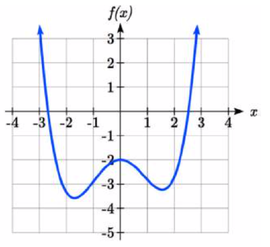
The vertex and end behavior allow us to determine where the parabola is increasing or decreasing as well as identify where the maximum or minimum value occurs. The real zeros of a parabola are the x-intercepts which help us determine where the function is positive or negative. With a larger polynomial, we seek to make a similar analysis. On the graph of the larger degree polynomial $f(x) = x^3 - x^2$ below,

$clipboard_efbe7d592c49c7d38d48fbde68e8d7e64.png$

the polynomial changes sign from positive to negative (or vice versus) at the real zeros (or x-intercepts) at $x=0$ and $x=1$ . The graph changes direction at $x = 0$ and $x \approx 0.67$ . Unlike a quadratic function, this third degree polynomial changes direction twice. Whereas a quadratic function has only one extrema, this polynomial has two relative extrema at the turning points where the graph changes direction. At the turning point $x=0$ , a relative maximum occurs. By a relative maximum, we mean that in a small interval containing $x=0$ , the function has its largest value in the interval at $x=0$ . At the turning point $x \approx 0.67$ , a relative minimum occurs. By a relative minimum, we mean that in a small interval containing $x\approx 0.67$ , the function has its smallest value in the interval at $x\approx 0.67$ . The relative maximum and minimums of a function are typically referred to as the relative extrema.

Definition: Relative Maximum

The function $y=f(x)$ has a relative maximum at x = a if $f(a) \ge f(x)$ for any $x$ in a small interval containing $x=a$ .

Definition: Relative Minimum

The function $y=f(x)$ has a relative minimum at x = a if $f(a) \le f(x)$ for any $x$ in a small interval containing $x=a$ .

Notice the end behavior of the polynomial: it opens up on the right (as $x \rightarrow + \infty , y \rightarrow + \infty$ ) and down on the left ( as $x \rightarrow - \infty , y \rightarrow - \infty$ ). These three features of the graph of a polynomial function will help us analyze the relationship it is describing.

Key Point: The Key Features of the Graph of a Polynomial Functions. $\PageIndex{1}$

The key features of the graph of a polynomial function are

The zeros
The relative extrema
The end behavior

In Calculus, we will explore techniques to locate the relative extreme. At this point in Precalculus, we will focus on identifying the zeros and the end behavior. We can use technology, such as a graphing calculator or graphing app, to approximate relative extrema on the graphs of polynomials at this point.

Focus: The Zeros of a Polynomial Function

As with quadratic functions, the zeros of polynomials are the values of $x$ for which the function value $f(x)=0$ . Real zeros are x-intercepts (or intercepts on the horizontal axis) on the graph. The zeros are a significant feature of a polynomial function since it will only change sign from positive to negative (or vice versus) at a real zero. Many of the techniques we used for solving polynomial equations in algebra will help us find the zeros of some polynomials.

Example $\PageIndex{2}$

Find the zeros of the polynomial functions.

$f(x)=x^3-x^2-6x$
$f(x)=x^4 +x^3 +x^2$

Solution

The zeros occur when $y=f(x)=0$ . So $x^3-x^2-6x=0\nonumber$ Factoring out a common factor of $x$ , then factoring the trinomial we have $x(x^2-x-6)=0\nonumber$ $x(x-3)(x+2)=0\nonumber$ The linear factors correspond to three distinct zeros $x=0, x=3, \text{and } x=2\nonumber$
Letting $y=f(x)=0$ , we have $x^4 +x^3 +x^2=0\nonumber$ Factoring out a common factor of $x^2$ $x^2(x^2+x+1)=0\nonumber$ Since the trinomial in not easily factorable into linear factors, we can set each factor to zero $x^2=x \cdot x = 0 \text{ and } x^2+x+1=0\nonumber$ In the first equation, we have two factors of $x$ that correspond to the zero $x=0$ . In the second equation, we must use the quadratic equation with $a=1$ , $b=1$ , and $c=1$ since the equation is not easily factored into linear factors. $x= \dfrac{-1 \pm \sqrt{1^2-4(1)(1)}}{2(1)}\nonumber$ $x= \dfrac{-1 \pm \sqrt{-3}}{2} = \dfrac{-1 \pm i \sqrt{3}}{2} = \dfrac{-1}{2} \pm i \dfrac{\sqrt{3}}{2}\nonumber$

Notice in the first polynomials in the previous example, we had three distinct real zeros that corresponding to a single linear factor each. Whereas in the second polynomial, we had a repeated real zero $x=0$ that correspond to two of the same linear factor as well as two complex zeros. In general, we could have a distinct real zero(s), a repeated zero(s), or complex conjugate zeros with a larger polynomial function. With quadratic functions, we had either two real zeros or two complex zeros. We need some language to describe the number of time a zero of a polynomial is repeated. We use call the number of linear factors $x-k)$ that corresponding to a zero $x=k$ the multiplicity off the zero.

Definition: The Multiplicity of a Zero

A zero $x=k$ of a polynomial $y=f(x$ has multiplicity $n$ if there are $n$ factors of the corresponding factor $x-k$ in the factorization of the polynomial.

Example $\PageIndex{3}$

Let $f(x)=x^5+4x^4+4x^3$ . Find the zeros and their multiplicity.

Solution

Letting $y=f(x)=0$ , we have $x^5+4x^4+4x^3=0\nonumber$ Factoring our a common factor of $x^3$ , then factoring the trinomial we have $x^3(x^2+4x+4)=0\nonumber$ $x^3(x+2)(x+2)=0\nonumber$ These factors correspond to the zeros $x=0$ with multiplicity three and $x=-2$ with multiplicity two.

Now you try: Exercise $\PageIndex{1}$

Let $f(x)=x^6-6x^5+9x^4$ . Find the zeros and their multiplicity.

Answer: $f(x)$ has zeros $x=0$ with multiplicity four and $x=3$ with multiplicity two.

Notice when finding the zeros and their multiplicities in each of the preceding examples and exercise, the polynomials had a common factor that when factored out of the polynomial, left a quadratic factor. When we set the quadratic factor to zero, we could solve with the quadratic formula or by factoring. With some larger polynomials, such as $f(x)=x^3-13x+12$ , there is no common factor. We can't use the quadratic formula since it is a cubic not a quadratic function. None of the techniques of solving polynomial equations from algebra help us find the zeros in this case. We will develop more tools in the next section to find the zeros of polynomials in this case.

As with quadratic functions, we can use the zeros of a polynomial and their multiplicities to find the formula for a polynomial function.

Example $\PageIndex{4}$

Find a formula for a polynomial function with zeros $x=1$ with multiplicity one and $x=-3$ with multiplicity two that passes through the point (0,4).

Solution

Since the polynomial has a zero $x=1$ with multiplicity one, there is a single factor of $x-1$ . Since the polynomial has a zero $x=-3$ with multiplicity two, there are two factors of $x+3$ . However, the polynomial $y=f(x)=(x-1)(x+3)^2$ passes through the point (0,-9) since $f(0) = -9$ . As with quadratic functions, the polynomial can also have a constant stretch factor $a$ . So $f(x)=a(x-1)(x+3)^2 \nonumber$ To find $a$ , we can substitute the point $x=0$ and $y=4$ into the polynomial $a(0-1)(0+3)^2=4 \nonumber$ Then solving for $a$ , we have $-9a=4 \nonumber$ $a=\dfrac{-4}{9} \nonumber$ Therefore, the formula for the polynomial is $f(x) =\dfrac{-4}{9}(x-1)(x+3)^2$

For our polynomial in example 4, we could leave our function in factored form as $f(x) =\dfrac{-4}{9}(x-1)(x+3)^2$ or multiply the factors out as $f(x) =\dfrac{-4}{9}x^3+\dfrac{20}{9}x^2-\dfrac{-4}{3}x+4$ . Depending on what we want to do with the formula for the polynomial, either form is useful.

Example $\PageIndex{5}$

Find a formula for a polynomial function with zeros $x=0$ with multiplicity three and $x=2i$ with multiplicity one that passes through the point (1,2).

Solution

Since the polynomial has a zero $x=0$ with multiplicity three, the polynomial has three factors of $x$ . Since the polynomial has the complex zero $x=2i$ of multiplicity one, the complex conjugate $x=-2i$ must also be a zero since complex zeros of polynomials appear in conjugate pairs. These complex zeros correspond to the factors $x-2i$ and $x+2i$ in the polynomial. Therefore, the polynomial has the formula $f(x)=ax^3(x-2i)(x+2i) \nonumber$ Simplifying by multiplying out the complex factors, we have $f(x)=ax^3(x^2-2ix+2ix-4i^2) \nonumber$ $f(x)=ax^3(x^2+4) \nonumber$ Subsituting the given point $x=1$ and $y=2$ into the polynomial to find the stretch factor $a$ then solving, we have $2=a1^3(1^2+4) \nonumber$ $2=5a \nonumber$ \[a=\dfrac{2}{5} \nonumber\. Therefore, the polynomial has a formula $f(x)=\dfrac{2}{5}x^3(x^2+4)$

Now You Try: Exercise $\PageIndex{2}$

Find a formula for a polynomial function with zeros $x=1$ with multiplicity one, $x=-2$ with multiplicity one, and $x=3$ with multiplicity two that passes through the point (0,5).

Answer: $f(x)=\dfrac{-5}{18}(x-1)(x+2)(x-3)^2$

Focus: The Behavior of the Graph of a Polynomial Function Near a Zero

As we have seen in the preceding examples, polynomial functions may have multiple distinct zeros each with a different multiplicity. Each real zero is an x-intercept. How does the multiplicity of a real zero affect the behavior of the graph near the zero? This is an important question we must address in order to graph larger polynomials.

Let's start by exploring the behavior of the graphs of powers of $x$ near the zero $x=0$ . If we graph the even even powers $y=x^2$ , $y=x^4$ , and $y=x^6$ on the same axis, notice the behavior of the graph near the zero at $x=0$ .

Each graph does not cross the x-axis at the zero.

Case: Powers of x

Let’s start by exploring the graphs of the odd powers $y=x^3$ , $y=x^5$ , and $y=x^7$ , near the zero $x=0$ .Notice each odd power has odd multiplicity for the zero $x=0$ (multiplicity three, five, and seven respectively). In the graph below, notice that each graph crosses the x-axis at the zero.

Try graphing larger odd powers such as $y=x^9$ and $y=x^11$ with your graph utility or app, notice that they also cross the x-axis at the zero.We can conclude that all odd powers will cross the x-axis at the zero.In general, the product of an odd number of factors of a positive number is positive whereas the product of an odd number of factors of a negative number is negative.Therefore, the odd power changes sign at the zero $x=0$ crossing the x-axis.

When we graph the even powers $y=x^2$ , $y=x^4$ , and $y=x^6$ , near the zero $x=0$ .Notice each even power has an even multiplicity for the zero $x=0$ (multiplicity two, four, and six respectively). In the graph below, notice that each graph does not cross the x-axis at the zero.Visually, it bounces off the x-axis as you move along the graph from right to left.Graphing larger even powers such as $y=x^8$ and $y=x^10$ with your graph utility or app, notice that they also do not cross the x-axis at the zero.We can conclude that all even powers will not cross the x-axis at the zero.In general, the product of an even number of factors of a positive number is positive and the product of an even number of factors of a negative number is positive also.Therefore, an even power does not change sign at the zero $x=0$ and does not cross the x-axis.

Key point:Odd powers of $x$ cross the x-axis at a zero $x=0$ .Even powers of $x$ do not cross the x-axis at the zero $x=0$

Next, let’s consider the scenario where we have a zero of $x=1$ . What happens as the multiplicity of the zero increases?

If the zero $x=1$ has multiplicity one, then a possible formula is $y=x-1$ .Notice, the line of slope $m=1$ crosses the x-axis at the zero.

If the zero $x=1$ has multiplicity two, then a possible formula is $y=(x-1)^2$ without a vertical stretch of reflection.The graph is a shift right one of the parabola $y=x^2$ which does not cross the x-axis at the zero. A vertical stretch or reflection will not change that the graph will not cross the x-axis at the zero.

If the zero $x=1$ has multiplicity three, then a possible formula is $y=(x-1)^3$ .The graph is a shift right one of the cubic $y=x^3$ which crosses the x-axis at the zero.

If the zero $x=1$ has multiplicity four, then a possible formula is $y=(x-1)^4$ .The graph is a shift right one of the even power $y=x^4$ which does not cross the x-axis at the zero.

If the zero $x=1$ has multiplicity five, then a possible formula is $y=(x-1)^5$ .The graph is a shift right one of the odd power $y=x^5$ . So the graph will cross the x-axis at the zero.

Case: the effect of multiple factors near a zero.

Consider the polynomial $y=x^3(x-1)$ where the zero $x=1$ has multiplicity one. As we near the zero $x=1$ from above, the factor (x-1) nears zero, the factor x^3 nears $x=1$ , so the product $y=x^3(x-1)$ nears $0 \cdot 1 = 0$ . Moreover, the other factor $x^3$ does not change sign at the zero $x=1$ , but $x-1$ does since it have odd multiplicity. Therefore, we can conclude the multiplicity of a real zero, determines the behavior of the graph near a real zero.

Key point: Real zeros of odd multiplicity will cross the x-axis at the real zero. Real zeros of even multiplicity will not cross the x-axis at the zero.

Without graphing with technology, determine whether the polynomial \(y=

intercepts and turning points of polynomials

A polynomial of degree $n$ will have:

At most $n$ horizontal intercepts. An odd degree polynomial will always have at least one.
At most $n - 1$ turning points

Example $\PageIndex{7}$

What can we conclude about the graph of the polynomial shown here?

$Polynomial graph decreasing to about (negative 1,7,negative 3.5), increasing to 0 comma negative 2, decreasing to 1.6 comma negative 3.2, then increasing.$

Solution

Based on the long run behavior, with the graph becoming large positive on both ends of the graph, we can determine that this is the graph of an even degree polynomial. The graph has 2 horizontal intercepts, suggesting a degree of 2 or greater, and 3 turning points, suggesting a degree of 4 or greater. Based on this, it would be reasonable to conclude that the degree is even and at least 4, so it is probably a fourth degree polynomial.

Exercise $\PageIndex{4}$

Given the function $f(x) = 0.2(x-2)(x+1)(x-5)$ , determine the short run behavior.

Answer: Horizontal intercepts are (2, 0) (-1, 0) and (5, 0), the vertical intercept is (0, 2) and there are 2 turns in the graph.

Short run Behavior: Intercepts

As with any function, the vertical intercept can be found by evaluating the function at an input of zero. Since this is evaluation, it is relatively easy to do it for a polynomial of any degree.

To find horizontal intercepts, we need to solve for when the output will be zero. For general polynomials, this can be a challenging prospect. While quadratics can be solved using the relatively simple quadratic formula, the corresponding formulas for cubic and 4 ${}^{th}$ degree polynomials are not simple enough to remember, and formulas do not exist for general higher-degree polynomials. Consequently, we will limit ourselves to three cases:

The polynomial can be factored using known methods: greatest common factor and trinomial factoring.
The polynomial is given in factored form.
Technology is used to determine the intercepts.

Other techniques for finding the intercepts of general polynomials will be explored in the next section.

Example $\PageIndex{1}$

Find the horizontal intercepts of $f(x)=x^{6} -3x^{4} +2x^{2}$ .

Solution

We can attempt to factor this polynomial to find solutions for $f(x) = 0$ .

$x^{6} -3x^{4} +2x^{2} =0\nonumber$ Factoring out the greatest common factor

$x^{2} (x^{4} -3x^{2} +2)=0\nonumber$ Factoring the inside as a quadratic in x ${}^{2}$

$x^{2} (x^{2} -1)(x^{2} -2)=0\nonumber$ Then break apart to find solutions

$\begin{array}{l} {x^{2} =0} \\ {x=0} \end{array}\text{ or }\begin{array}{l} {\left(x^{2} -1\right)=0} \\ {x^{2} =1} \\ {x=\pm 1} \end{array}\text{ or }\begin{array}{l} {\left(x^{2} -2\right)=0} \\ {x^{2} =2} \\ {x=\pm \sqrt{2} } \end{array}\nonumber$

This gives us 5 horizontal intercepts.

Example $\PageIndex{2}$

Find the vertical and horizontal intercepts of $g(t)=(t-2)^{2} (2t+3)$

Solution

The vertical intercept can be found by evaluating $g(0)$ .

$g(0)=(0-2)^{2} (2(0)+3)=12\nonumber$

The horizontal intercepts can be found by solving $g(t) = 0$

$(t-2)^{2} (2t+3)=0\nonumber$ Since this is already factored, we can break it apart:

$\begin{array}{l} {(t-2)^{2} =0} \\ {t-2=0} \\ {t=2} \end{array}\text{ or }\begin{array}{l} {(2t+3)=0} \\ {t=\dfrac{-3}{2} } \end{array}\nonumber$

We can always check our answers are reasonable by graphing the polynomial.

Example $\PageIndex{3}$

Find the horizontal intercepts of $h(t)=t^{3} +4t^{2} +t-6$

Solution

$A polynomial that increases, decreases, then increases, with apparent horizontal intercepts at negative 3 comma 0, negative 2 comma 0 and 1 comma 0$ Since this polynomial is not in factored form, has no common factors, and does not appear to be factorable using techniques we know, we can turn to technology to find the intercepts.

Graphing this function, it appears there are horizontal intercepts at $t$ = -3, -2, and 1.

We could check these are correct by plugging in these values for t and verifying that $h(-3)=h(-2)=h(1)=0$ .

Exercise $\PageIndex{1}$

Find the vertical and horizontal intercepts of the function $f(t)=t^{4} -4t^{2}$ .

Answer: Vertical intercept (0, 0). $0=t^{4} -4t^{2}$ factors as $0=t^{2} \left(t^{2} -4\right)=t^{2} \left(t-2\right)\left(t+2\right)$ Horizontal intercepts (0, 0), (-2, 0), (2, 0).

Graphical Behavior at

Important Topics of this Section

Power Functions
Polynomials
Coefficients
Leading coefficient
Term
Leading Term
Degree of a polynomial
Long run behavior
Short run behavior