2.2: Modeling with Exponential Functions

Goal: Describing relationships with exponential functions.

Case: The growth factor is given.

Example \(\PageIndex{1}\)

When an outbreak of a contagious virus was first discovered, there were 1200 cases. Each week the number of cases triples.

a) Find a formula for the number of cases, C, in t weeks since the virus was discovered. Then sketch a graph.

b) Predict the number of cases in 3 months if the cases continue to grow in this manner.

Solution

a) The initial value a = 1200 and the growth factor b = 3 since we are multiplying the number of cases by 3 for each week. Using \( y=a(b)^{x} \) or \(C=a(b)^{t} \), our formula is \(C=1200(3)^{t} \). To sketch the graph, we know the function is increasing since \( b = 3 > 1\) and the y-intercept is at y = 1200 since a = 1200.

b) The number of cases in 3 month is \(C=1200(3)^{3} = 32,400. \)

Case: Functions with a constant percentage rate of change.

Example \(\PageIndex{2}\)

Suppose you invest $1000 at a 6% annual interest rate compounded annually.

a) Is this exponential growth?

b) Find a formula for the amount in the account, A, in t years. Then sketch a graph.

c) Predict the amount in the account after 10 years.

Solution

a) After one year, the amount in the account will be

the original amount (100%) + interest (6%) = 106% of the original amount = \(1.06(1000)\)=$1060.

After the second year, the account will have 106% of the previous years amount of $1060 or \[1.06(1060) = (1.06)(1.06)(1000) = (1.06)^{2}(1000) = 1,123.60 \nonumber\] by the same rationale. Each subsequent year, the account will have 106% of the previous years amount = 100% (previous years amount) + 6% (interest). This is exponential growth since we are multiplying the output A by a growth factor b = 1.06 for each increase in x by 1 \( (\Delta x = 1) \) as illustrated in the table below.

Years invested, t	0	1	2	3	4
Amount in the account, A	\( $1000 \)	\(1,000(1.06)^{1}\\ = $1,060\)	\(1,060(1.06) \\ = 1,000(1.06)^{2} \\ = $1,123.60\)	\(1,123.60(1.06)\\ = 1,000(1.06)^{3} \\ = $1,191.02\)	\(1,191.02(1.06) \\ = 1,000(1.06)^{4} \\ = $1,262.48\)

b) The growth factor is b = 1.06. The initial value is a = $1000. So the formula for the amount in the account in t years is given by \[A = 1,000(1.06)^{t} \nonumber\] To sketch the graph, we know the function is increasing since \( b = 1.06 > 1\) and the vertical intercept or A-intercept is at A = 1000 since a = 1000.

c) In ten years (t = 10), the amount is predicted to be \[A= 1,000(1.06)^{10} = $1,790.85 \nonumber\] .

Notice that the growth factor b = 1.06 = 1.00 + 0.06 as decimal or b = 106% = 100% + 6%.

Example \(\PageIndex{3}\)

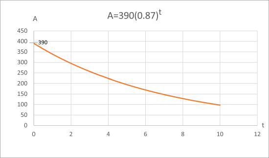
A person drinks three cups of coffee containing 390 mg of caffeine. Suppose their body eliminates 13% of the caffeine each hour.

a) Is this exponential decay?

b) Find a formula for the amount in the caffeine, A, in t hours. Then sketch a graph.

c) Predict the amount of caffeine after 6 hours.

Solution

a) After one hour, the amount of caffeine in the body will be

(the original amount (100%)) - (amount eliminated (13%)) = 87% of the original amount = \(0.87(390)\)= 339.3 mg of caffeine.

After the second year, the amount in the body will have 87% of the previous hour's caffeine level of 339.3 mg or \[0.87(339.3) = (0.87)(0.87)(390) = 390(0.87)^{2} \nonumber\] by the same rationale. Each subsequent hour, the amount in the body will have

87% of the previous hour's caffeine level = 100% (previous hour's caffeine level) - 13% (amount eliminated).

This is exponential decay since we are multiplying the output A by a growth factor b = 0.87 for each increase in x by 1 \( (\Delta x = 1) \) as illustrated in the table below.

t hours since the coffee was ingested	0	1	2	3	4
A, the amount of caffeine in the body in mg	\( 390 \text { mg }\)	\(390(0.87)^{1} \\ = 339.3 \text { mg } \)	\(339.3(0.87) \\ = 390(0.87)^{2} \\ = 295.19 \text{ mg } \)	\(295.19(0.87) \\ = 390(0.87)^{3} \\ = 256.82 \text{ mg } \)	\(256.82(0.87) \\ = 390(0.87)^{4} \\ = 223.43 \text{ mg }\)

b) The growth factor is b = 0.87. The initial value is a = $390 mg. So the formula for the amount in the account in t hours is given by \[A = 390(0.87)^{t}. \nonumber\] To sketch the graph, we know the function is decreasing since \( b = 0.87 < 1\) and the vertical intercept or A-intercept is at A = 390 since a = 390.

c) In six hours (t = 6), the amount of caffeine in the body is predicted to be \[A= 390(0.87)^{6} = 169.11 \, mg \nonumber\] .

Notice that the growth factor b = 0.87 = 1.00 - 0.13 as decimal or b = 87% = 100% - 13%.

Key Point

A quantity that changes by a constant percentage rate r relative to a another quantity x is experiencing exponential growth (or decay) with a growth factor

b = 100% + r% (as a percent) or b = 1 + r (as a decimal).

Example \(\PageIndex{4}\)

India is the second most populous country in the world, with a population in 2008 of about 1.14 billion people. The population is growing by about 1.34% each year (World Bank, World Development Indicators, as reported on http://www.google.com/publicdata, retrieved August 20, 2010).

a) Find a formula to model the population of India, \(P\), as a function of time, \(t\), in years after 2008, if the population continues to grow at this rate.

b) Predict the population of India in 2030 if it continues to grow at this rate.

Solution

a) The growth factor is b = 100% + 1.34% = 101.34% as a percent or b = 1 + 0.0134 = 1.0134 as a decimal. The initial value is a = 1.14 billion people. The formula for the population t years after 2008 is given by \[P= 1.14(1.0134)^{t} \nonumber\]

b) The population in 2030 (t = 22 years after 2008) is predicted to be \[P= 1.14(1.0134)^{22}=1.52 \text{ billion people.} \nonumber\]

Example \(\PageIndex{5}\)

\(T(q)\) represents the total number of Android smart phone contracts, in thousands, held by a certain Verizon store region \(q \) quarters since January 1, 2016, interpret all the parts of the equation \(T(2)=86(1.64)^{2} =231.3056\).

Solution

Interpreting this from the basic exponential form, we know that 86 is our initial value. This means that on Jan. 1, 2016 this region had 86,000 Android smart phone contracts. Since \(b = 1 + r = 1.64\), we know that every quarter the number of smart phone contracts grows by 64%. \(T(2) = 231.3056\) means that in the \(2^{nd}\) quarter (or at the end of the second quarter) there were approximately 231,306 Android smart phone contracts.

Student Exercise \(\PageIndex{1}\)

The number of students at Clovis Community College was 10,092 in the Fall 2014 semester. Over the next few years, the number of students grew by approximately 8% per year (reported by The Clovis Community College Institutional Research Department). Assume the number of students continues to grow at this rate.

a) Write an exponential function for the number of students, S, at Clovis Community College t years after the Fall 2014 if the student population continues to grow in this manner.

b) Predict the number of students at Clovis Community College in the fall 2025 semester.

Answer

a) The growth factor is b = 100% + 8% = 108% as a percent or b = 1 + 0.08 = 1.08 as a decimal. The initial value is a = 10,092 students. The formula for the number of students t years after 2014 is given by \[S = 10,091(1.08)^{t} \nonumber\]

b) The number of students in the Fall 2025 semester (t = 11) is predicted to be \[S = 10,091(1.08)^{11} =23,530 \, students \nonumber\]

Student Exercise \(\PageIndex{2}\)

Given the three statements below, identify which represent exponential functions.

1. The cost of living allowance for state employees increases salaries by 3.1% each year.
2. State employees can expect a $300 raise each year they work for the state.
3. Tuition costs have increased by 2.8% each year for the last 3 years.

Answer

a & c are exponential functions, they grow by a % not a constant number.

Student Exercise \(\PageIndex{3}\)

Looking at these two equations that represent the balance in two different savings accounts, which account is growing faster, and which account will have a higher balance after 3 years?

• \(A(t)=1000\left(1.05\right)^{t}\)
• \(B(t)=900\left(1.075\right)^{t}\)

Answer

\(B(t)\) is growing faster (\(r\) = 0.075 > 0.05), but after 3 years A(t) still has a higher account balance since \[A(3) = $1157.63 > B(3) = $1,118.07 \nonumber \]

Exponential functions can be used to model quantities that are decreasing at a constant percent rate as we saw in example 3.2.2. Another example of this is radioactive decay, a process in which radioactive isotopes of certain atoms transform to an atom of a different type, causing a percentage decrease of the original material over time.

Student Exercise \(\PageIndex{4}\)

Bismuth-210 is an isotope that radioactively decays each day, meaning a part of the remaining Bismuth-210 transforms into another atom (polonium-210 in this case) each day. If \(Q(d) \) represents the amount of Bismuth-210 remaining in \(d \) days, interpret the meaning of the formula \[Q(d)=100(1-0.13)^{d} =100(0.87)^{d}.\nonumber\]

Answer

The growth factor b = 0.87 = 1 - 0.13 tells use the amount of the isotope is decreasing by 13% percent each hour. Our initial quantity is \(a\) = 100 mg of Bismuth-210.

Case: Finding Equations of Exponential Functions from Data

In the previous examples, we were able to write formula for exponential functions since we knew the initial quantity and the growth rate. However, in many cases, we will be able to measure or collect data on exponentially growing (or decaying) quantities. We can use this to construct exponential functions that describe these relationships.

In our original examples in section 3.1, we were given data sets with consecutive values of the input. For example, in the table from student exercise 3.1.1, we are able to easily identify the growth factor b = 4, since b is the value we multiply each output by for each increase in x by 1.

x	0	1	2	3	4
\(f(x)\)	3	12	48	192	7687

What is the difference in the following table of data? Is the growth factor b = 4 also?

x	0	3	6	9	12
\(f(x)\)	3	12	48	192	7687

Notice that x is increasing by 3 \( ( \Delta x =3) \) instead of by 1. The growth factor is the number we multiply the output by for each increase in x by 1. In this case for \( ( \Delta x =3) \), we would have to multiply the output by the growth factor three times. To model the data with an exponential function, we can use the fact that our initial value a = 3 and the point x = 3, y =12 is a solution to our exponential equation described by our function \(y=ab^{x}\).

Substituting in a = 3 and the point (x,y) = (3, 12) gives \(12=3b^{3}\).

Solving for \(a\) we have,

\[\begin{array}{l} {12=3b^{3} } \\ {\dfrac{12}{3}=b^{3} } \\ {4=b^{3} } \\ {b=\sqrt[{3}]{4} \approx 1.5974} \end{array}\nonumber\]

Example 3.2.6

Find a formula for an exponential function passing through the points (0,6) and (5,1).

Solution

The initial value of the function and y-intercept on the graph is at y = 6 so a = 6. Now the point x = 5, y =1 is a solution to our exponential equation described by our function \(y=ab^{x}\).

Substituting in a = 6 and the point (x,y) = (5, 1) gives \(1=6b^{5}\).

Solving for \(a\) we have,

\[\begin{array}{l} {1=6b^{5} } \\ {\dfrac{1}{6}=b^{5} } \\ {b=\sqrt[{5}]{\dfrac{1}{6}} \approx 0.6988} \end{array}\nonumber\]

So the formula for the exponential function that models this data is given by \(f(x) \approx 6(0.6988)^{t}.\)

In this example, you could also have used \((\dfrac{1}{6})^{\dfrac{1}{5}}\) to evaluate the 5\({}^{th}\) root if your calculator doesn’t have an \({n}^{th}\) root button.

Example \(\PageIndex{7}\)

Find a formula for an exponential function passing through the points (1,6) and (5,1).

Solution

What is the difference with this problem and the previous one? We don't know the initial value of the function or y-intercept on the graph since x = 1 when y = 6. However, we can use the same strategy we used with the other point. Since the point x = 5, y =1 is a solution to our exponential equation \(y=ab^{x}\), we can substitute these values into the the equation so that \(1=ab^{5}\).

This is an equation in terms of two variables. We need a second independent equation in order to solve this system of equations. With the second point (1,6), we can substitute x= 1 and y =6. This gives \(6=ab^{1}\).

We now solve these as a system of equations. \[\begin{array}{l} {1=ab^{5} } \\ {6=ab^{1} } \end{array}\nonumber\]

To do so, we can use a substitution method by solving for the variable \(a\) in the second equation \(6=ab^{1}\). .

So we have, \[a= \dfrac{6}{b^{1}}. \nonumber\]

Then substituting the expression for \(a\) into the second equation \(1=ab^{5}\):

\[\begin{array}{l} {1=\dfrac{6}{b^{1}}(b^{5})} \\ {1=6b^{4} } \\ {\dfrac{1}{6} =b^{4} } \\ {b=\sqrt[{4}]{\dfrac{1}{6} } \approx 0.6988} \end{array}\nonumber\]

Going back to the equation \(a= \dfrac{6}{b^{1}}\) lets us find \(a\):

\[a= \dfrac{6}{0.6389} \approx 8.586\nonumber\]

Putting this together gives the formula \(f(x) \approx 8.586(0.6389)^{x}\)

Notice how much easier it was to find the formula for the exponential function when the initial value a (or y-intercept on the graph) is known. We only need to solve a single equation to find b in example 3.2.6 as opposed to a system of equations in example 3.2.7 when the initial value a is not known. In many applications, it is possible and makes sense to define our variables so that the first data point is the initial value. For example in student example 3.2.1, we defined t as the years after the fall 2014 which made the first data point (the number of students was 10,092 in Fall 2014) an initial value t = 0 and S = 10,092.

Case: Finding Equations of Exponential Functions in Applications

Example \(\PageIndex{8}\)

On December 12, 2021, the number of new daily Covid cases in the US was 119,221 (represented as a 7-day average as reported by the Center for Disease Control (CDC) at covid.cdc.gov). By December 30, 2021 , the number of new daily US Covid cases rose to 364,369. Additional data in this time frame show the numbers of cases were increasing at an increasing rate. Assume the number of daily Covid cases is growing exponentially.

a) Find a formula for the number of new daily Covid cases, C, t days since Dec. 12, 2021.

b) Predict the number of new Covid cases on Jan. 10, 2021 if this trend continues.

Solution

a) By defining our input variable to be \(t\) days since Dec. 12, 2021, the information listed can be written as two input-output pairs: t = 0, C = 119,221 and t = 18, C = 364,369. Notice that by choosing our input variable to be measured as the days after the first day value provided, we have effectively “given” ourselves the initial value for the function: \(a\) = 119,221. This gives us an equation of the form

\[C=f(t)=119,221b^{t} \nonumber\]

Substituting in our second input-output pair allows us to solve for \(b\):

\[364,369=119,221b^{18}\nonumber\] Dividing by 119,221.
\[b^{18} =\dfrac{364,369}{119,221} \approx 3.05625 \nonumber\] Take the 18\({}^{th}\) root of both sides.
\[b=\sqrt[{18}]{3.05625 } \approx 1.06403 \nonumber\]

This gives us our equation for the number of new daily Covid cases:

\[C=f(t)=119,221(1.06403)^{t}\nonumber\]

Recall that since \(b = 1+r\), we can interpret this to mean that the daily new Covid cases' growth rate is \(r\) = 0.06403, and so the daily new Covid cases' is growing by about 6.4303% each day.

b) Jan. 10, 2022 represents t = 29 days since Dec. 12, 2021. Using our formula, the number of new Covid cases (as a 7-day average) on this day is

\[C=f(29)=119,221(1.06403)^{29} \approx 721,132.\nonumber\]

Note that the actual number of cases on this day as a 7-day average was 760,924.

When finding equations, the value for \(b\) or \(r\) will usually have to be rounded to be written easily. To preserve accuracy, it is important to not over-round these values. Typically, you want to be sure to preserve at least 3 or 4 significant digits in the growth rate. For example, if your value for \(b\) was 1.064032579, you would want to round this no further than to 1.06403 or 1.0640.

Example \(\PageIndex{9}\)

In 1981, the five year average daily maximum temperature in Fresno, County was 67.41 \(^{o}\)F. In 2011, the five year average daily maximum temperature rose to 69.13 \(^{o}\)F. Assume the five year average daily maximum temperature increases exponentially. (Data collected by North America Land Data Assimilation System (NLDAS) and reported on wonder.cdc.gov)

a) Find an exponential model for the five year average daily maximum temperature in Fresno, County, T, in t years since 1981.

b) Use your model to predict the five year average daily maximum temperature in Fresno, County in 2026 assuming the temperatures continue to increase in this manner.

Solution

a) By defining our input variable to be \(t\), years after 1981, the information listed can be written as two input-output pairs: t = 0, T = 67.41 and t = 20, T = 69.13 Notice that by choosing our input variable to be measured as years after the first year value provided, we have effectively “given” ourselves the initial value for the function: \(a\) = 67.41. This gives us an equation of the form

\[T=f(t)=67.41b^{t} \nonumber\]

Substituting in our second input-output pair allows us to solve for \(b\):

\[69.13=67.41b^{20}\nonumber\] Divide by 67.41
\[b^{20} =\dfrac{69.13}{67.41} \approx 1.025516\nonumber\] Take the 20\({}^{th}\) root of both sides.
\[b=\sqrt[{20}]{1.025516 } \approx 1.0012603\nonumber\]

This gives us our equation for the the five year average daily maximum temperature in Fresno County:

\[T=f(t)=67.41(1.0012603)^{t}\nonumber\]

Recall that since \(b = 1+r\), we can interpret this to mean that the five year average daily maximum temperature in Fresno County is growing by about 0.12603% each year.

b) In 2026, t = 45 years since 1981. Substituting this value in for t in our formula

\[T=f(t)=67.41(1.0012603)^{45} \approx 71.34 ^{o}F \nonumber\]

Another important application of exponential functions in physics, chemistry, engineering, and biology is radioactive decay. Radioactive decay is the idea that the amount of radioactive isotopes decreases exponentially over time. One of the common terms associated with radioactive decay is half-life.

Definition: Half Life

The half-life of a radioactive isotope is the time it takes for half or 50% of the substance to decay.

Example \(\PageIndex{10}\)

Cesium-137 is a radioactive compound that has a half-life of about 30 years. It is a common waste product in the production of nuclear energy. A sample is taken near a nuclear accident that contains 200 mg of cesium-137.

a) Find a formula for the amount of Cesium-137, C, of the sample in t years.

b) Predict the amount of Cesium in the sample in 50 years.

Solution

a) By defining our input variable to be \(t\) years since the sample was taken, the initial value is t = 0, C = 200 mg. Notice that by choosing our input variable to be measured as years after the first year value provided, we have effectively “given” ourselves the initial value for the function: \(a\) = 200. This gives us an equation of the form

\[C=f(t)=200b^{t} \nonumber\]

The half life can be used to obtain a second data point. In 30 years (t=30), there is half or 50% of the original amount remaining. So C = (0.50)(200) = 100 mg. Substituting this data into out formula allows us to solve for \(b\):

\[100=200b^{30}\nonumber\] Divide by 200
\[b^{30} =\dfrac{100}{200} =0.5 \nonumber\] Take the 30\({}^{th}\) root of both sides.
\[b=\sqrt[{30}]{0.5 } \approx 0.97716\nonumber\]

This gives us our equation for the amount of Cesium:

\[C=f(t)=200(0.97716)^{t}\nonumber\]

Recall that since \(b = 1+r\), so \(r = b - 1 = 0.97716 - 1 = -0.0228\) or \(r\) = -2.284%. We can interpret this to mean that the amount of cesium is decreasing by about 2.284% each year.

b) In 50 years, t = 50. Substituting this value in for t in our formula

\[T=f(t)=200(0.97716)^{50} \approx 62.997 \text{ mg} \nonumber\]

Student Exercise \(\PageIndex{5}\)

The number of students at Clovis Community College was 10,092 in the Fall 2014 semester. By the Fall 2019 semester, the number of students as 14,384 (as reported by The Clovis Community College Institutional Research Department). Assume the number of students grows exponentially.

a) Write an exponential function for the number of students, S, at Clovis Community College t years after the Fall 2014 semester, if the student population continues to grow in this way.

b) Predict the number of students at Clovis Community College in the fall 2025 semester.

Answer

a) By defining our input variable to be \(t\), years after the Fall 2014 semester, the information listed can be written as two input-output pairs: t = 0, S = 10092 and t = 5, S = 14,384. Notice that by choosing our input variable to be measured as years after the first year value provided, we have effectively “given” ourselves the initial value for the function: \(a\) = 10,092. This gives us an equation of the form

\[S=f(t)=10,092b^{t} \nonumber\]

Substituting in our second input-output pair allows us to solve for \(b\):

\[14,384=10,092b^{5}\nonumber\] Divide by 10,092
\[b^{5} =\dfrac{14,384}{10,092} \approx 1.4253\nonumber\] Take the 5\({}^{th}\) root of both sides.
\[b=\sqrt[{5}]{1.4253 } \approx 1.0734\nonumber\]

This gives us our equation for the number of students at Clovis Cummunity College:

\[S=f(t)=10092(1.0734)^{t}\nonumber\]

Recall that since \(b = 1+r\), we can interpret this to mean that the of number of students is growing by about 7.34% each year.

b) In fall 2025, t = 11 years since the Fall 2014 semester. Substituting this value in for t in our formula

\[S=f(t)=10092(1.0734)^{11} \approx 21,997 \text{ students}. \nonumber\]

Student Exercise \(\PageIndex{6}\)

Carbon-14 is a radioactive isotope that is present in organic materials, and is commonly used for dating historical artifacts. Carbon-14 has a half-life of 5730 years.

a) Find a formula for the percentage, P, of the original carbon-14 remaining.

b) If the bone is 10,000 years old, what percentage of the original carbon-14 remains?

Answer

a) Let define \(t\) = age of the bone in years. Then, the half-life can be interpretted as an input-output pair:

t = 5,730 years, P = 50%. Although it is not stated explicitly in the problem, we do know a second data point: when the animal died (time t= 0) there is 100% of the original carbon -14 remaining (P=100). This gives us initial value for the function: \(a\) = 100. This gives us an equation of the form

\[S=f(t)=100b^{t} \nonumber\]

Substituting in our other input-output pair allows us to solve for \(b\):

\[50=100b^{5730}\nonumber\] Divide by 100
\[b^{5730} =\dfrac{50}{100} =0.5\nonumber\] Take the 5730\({}^{th}\) root of both sides.
\[b=\sqrt[{5730}]{0.5 } \approx 0.999879\nonumber\]

This gives us our equation for the percentage of the original carbon-14 remaining:

\[P=f(t)=100(0.999879)^{t}\nonumber\]

b) If the bone is 10,000 years old, then t = 10,000. Substituting this value in for t in our formula

\[P=f(t)=100(0.999879)^{10000} \approx 29.83 \text{% of the original carbon-14 remains.} \nonumber\]

Important Topics of this Section

• Percent growth
• Exponential functions
• Finding formulas
• Interpreting equations
• Exponential Growth & Decay
• Radioactive decay
• Half life