4.3: Graphing Polynomial Functions

Last updated
Save as PDF

Page ID: 99734

$ \newcommand{\vecs}[1]{\overset { \scriptstyle \rightharpoonup} {\mathbf{#1}} } $

$ \newcommand{\vecd}[1]{\overset{-\!-\!\rightharpoonup}{\vphantom{a}\smash {#1}}} $

$ \newcommand{\dsum}{\displaystyle\sum\limits} $

$ \newcommand{\dint}{\displaystyle\int\limits} $

$ \newcommand{\dlim}{\displaystyle\lim\limits} $

$ \newcommand{\id}{\mathrm{id}}$ $ \newcommand{\Span}{\mathrm{span}}$

( \newcommand{\kernel}{\mathrm{null}\,}\) $ \newcommand{\range}{\mathrm{range}\,}$

$ \newcommand{\RealPart}{\mathrm{Re}}$ $ \newcommand{\ImaginaryPart}{\mathrm{Im}}$

$ \newcommand{\Argument}{\mathrm{Arg}}$ $ \newcommand{\norm}[1]{\| #1 \|}$

$ \newcommand{\inner}[2]{\langle #1, #2 \rangle}$

$ \newcommand{\Span}{\mathrm{span}}$

$ \newcommand{\id}{\mathrm{id}}$

$ \newcommand{\Span}{\mathrm{span}}$

$ \newcommand{\kernel}{\mathrm{null}\,}$

$ \newcommand{\range}{\mathrm{range}\,}$

$ \newcommand{\RealPart}{\mathrm{Re}}$

$ \newcommand{\ImaginaryPart}{\mathrm{Im}}$

$ \newcommand{\Argument}{\mathrm{Arg}}$

$ \newcommand{\norm}[1]{\| #1 \|}$

$ \newcommand{\inner}[2]{\langle #1, #2 \rangle}$

$ \newcommand{\Span}{\mathrm{span}}$ $ \newcommand{\AA}{\unicode[.8,0]{x212B}}$

$ \newcommand{\vectorA}[1]{\vec{#1}} % arrow$

$ \newcommand{\vectorAt}[1]{\vec{\text{#1}}} % arrow$

$ \newcommand{\vectorB}[1]{\overset { \scriptstyle \rightharpoonup} {\mathbf{#1}} } $

$ \newcommand{\vectorC}[1]{\textbf{#1}} $

$ \newcommand{\vectorD}[1]{\overrightarrow{#1}} $

$ \newcommand{\vectorDt}[1]{\overrightarrow{\text{#1}}} $

$ \newcommand{\vectE}[1]{\overset{-\!-\!\rightharpoonup}{\vphantom{a}\smash{\mathbf {#1}}}} $

$ \newcommand{\vecs}[1]{\overset { \scriptstyle \rightharpoonup} {\mathbf{#1}} } $

$\newcommand{\longvect}{\overrightarrow}$

$ \newcommand{\vecd}[1]{\overset{-\!-\!\rightharpoonup}{\vphantom{a}\smash {#1}}} $

$\newcommand{\avec}{\mathbf a}$ $\newcommand{\bvec}{\mathbf b}$ $\newcommand{\cvec}{\mathbf c}$ $\newcommand{\dvec}{\mathbf d}$ $\newcommand{\dtil}{\widetilde{\mathbf d}}$ $\newcommand{\evec}{\mathbf e}$ $\newcommand{\fvec}{\mathbf f}$ $\newcommand{\nvec}{\mathbf n}$ $\newcommand{\pvec}{\mathbf p}$ $\newcommand{\qvec}{\mathbf q}$ $\newcommand{\svec}{\mathbf s}$ $\newcommand{\tvec}{\mathbf t}$ $\newcommand{\uvec}{\mathbf u}$ $\newcommand{\vvec}{\mathbf v}$ $\newcommand{\wvec}{\mathbf w}$ $\newcommand{\xvec}{\mathbf x}$ $\newcommand{\yvec}{\mathbf y}$ $\newcommand{\zvec}{\mathbf z}$ $\newcommand{\rvec}{\mathbf r}$ $\newcommand{\mvec}{\mathbf m}$ $\newcommand{\zerovec}{\mathbf 0}$ $\newcommand{\onevec}{\mathbf 1}$ $\newcommand{\real}{\mathbb R}$ $\newcommand{\twovec}[2]{\left[\begin{array}{r}#1 \\ #2 \end{array}\right]}$ $\newcommand{\ctwovec}[2]{\left[\begin{array}{c}#1 \\ #2 \end{array}\right]}$ $\newcommand{\threevec}[3]{\left[\begin{array}{r}#1 \\ #2 \\ #3 \end{array}\right]}$ $\newcommand{\cthreevec}[3]{\left[\begin{array}{c}#1 \\ #2 \\ #3 \end{array}\right]}$ $\newcommand{\fourvec}[4]{\left[\begin{array}{r}#1 \\ #2 \\ #3 \\ #4 \end{array}\right]}$ $\newcommand{\cfourvec}[4]{\left[\begin{array}{c}#1 \\ #2 \\ #3 \\ #4 \end{array}\right]}$ $\newcommand{\fivevec}[5]{\left[\begin{array}{r}#1 \\ #2 \\ #3 \\ #4 \\ #5 \\ \end{array}\right]}$ $\newcommand{\cfivevec}[5]{\left[\begin{array}{c}#1 \\ #2 \\ #3 \\ #4 \\ #5 \\ \end{array}\right]}$ $\newcommand{\mattwo}[4]{\left[\begin{array}{rr}#1 \amp #2 \\ #3 \amp #4 \\ \end{array}\right]}$ $\newcommand{\laspan}[1]{\text{Span}\{#1\}}$ $\newcommand{\bcal}{\cal B}$ $\newcommand{\ccal}{\cal C}$ $\newcommand{\scal}{\cal S}$ $\newcommand{\wcal}{\cal W}$ $\newcommand{\ecal}{\cal E}$ $\newcommand{\coords}[2]{\left\{#1\right\}_{#2}}$ $\newcommand{\gray}[1]{\color{gray}{#1}}$ $\newcommand{\lgray}[1]{\color{lightgray}{#1}}$ $\newcommand{\rank}{\operatorname{rank}}$ $\newcommand{\row}{\text{Row}}$ $\newcommand{\col}{\text{Col}}$ $\renewcommand{\row}{\text{Row}}$ $\newcommand{\nul}{\text{Nul}}$ $\newcommand{\var}{\text{Var}}$ $\newcommand{\corr}{\text{corr}}$ $\newcommand{\len}[1]{\left|#1\right|}$ $\newcommand{\bbar}{\overline{\bvec}}$ $\newcommand{\bhat}{\widehat{\bvec}}$ $\newcommand{\bperp}{\bvec^\perp}$ $\newcommand{\xhat}{\widehat{\xvec}}$ $\newcommand{\vhat}{\widehat{\vvec}}$ $\newcommand{\uhat}{\widehat{\uvec}}$ $\newcommand{\what}{\widehat{\wvec}}$ $\newcommand{\Sighat}{\widehat{\Sigma}}$ $\newcommand{\lt}{<}$ $\newcommand{\gt}{>}$ $\newcommand{\amp}{&}$ $\definecolor{fillinmathshade}{gray}{0.9}$

In this section, our goal is to graph polynomial functions. As we did with quadratic functions in sections 3.2 and 3.3, we will use the key features of a polynomial to graph it. We learned in sections 4.1 and 4.2 how to find the zeros of a polynomial function. We will also need to determine the end behavior of a larger polynomial in order to graph the polynomial. As well, we need to understand the effect of the multiplicity of real zero on the behavior of the graph near that zero.

Focus: Determining The End Behavior of a Larger Polynomial Functions

Case: The End Behavior of Powers of $x$, $y=x^n$

When we graph the even powers $y=x^2$, $y=x^4$, and $y=x^6$ on the same axis below, notice that although the graphs flatten somewhat near the origin, and become steeper away from the origin as the power increases, they all have the same end behavior. All the graphs open up on both ends, just like the parabola $y=x^2$. As we highlighted with quadratic functions in Chapter 3, when we say the graph opens up on the right end, we mean as $x \to \infty$, $y \to \infty$. When we say the graph opens up on the left end, we mean as $x \to -\infty$, $y \to \infty$.

$The graph of three even powers which open up on both ends$

If you graph larger even powers, such as $y=x^8$ and $y=x^{10}$, you will find the same end behavior as $y=x^2$. By extension, we can conclude all even powers of $x$ will have the same end behavior as the parabola $y=x^2$, opening up on both ends (as $x \to \pm \infty$, $y \to \infty$).

When we graph the odd powers $y=x^3$, $y=x^5$, and $y=x^7$ on the same axis below, notice that they all have the same end behavior. The graphs open up on the right end (as $x \to \infty$, $y \to \infty$) and down on the left end (as $x \to - \infty$, $y \to -\infty$)

$The graphs of three odd powers which open up on the right and down on the left.$

If you graph larger odd powers, such as $y=x^9$ and $y=x^{11}$, you will find the same end behavior as $y=x^3$. By extension, we can conclude all odd powers of $x$ will have the same end behavior as the cubic $y=x^3$, open up on the right end (as $x \to \infty$, $y \to \infty$) and down on the left end (as $x \to - \infty$, $y \to -\infty$).

Key Point $\PageIndex{1}$: The End Behavior of Powers of $x$

For the power functions $y=x^n$, all even powers of $x$ will have the same end behavior as the parabola $y=x^2$, opening up on both ends (as $x \to \pm \infty$, $y \to \infty$). All odd powers of $x$ will have the same end behavior as the cubic $y=x^3$, open up on the right end (as $x \to \infty$, $y \to \infty$) and down on the left end (as $x \to - \infty$, $y \to -\infty$).

Case: The End Behavior of Power Functions of the Form $y=ax^n$

What is the effect of the stretch factor $a$ on the end behavior? Consider the graphs of $y=x^2$, $y=2x^2$, and $y=-2x^2$ below with stretch factors $a=1$, $a = 2$, and $a=-2$ respectively.

$The graph of the parabola y = x^2 and a second parabola with a vertical stretch.$ $The graph of a parabola and its reflection.$

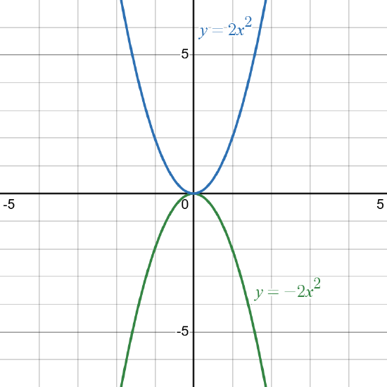
Notice with the graph of $y=2x^2$ in the graph on the left, the stretch factor $a=2$ causes a vertical stretch by a factor of two on the graph of $y=x^2$. The vertical stretch does not change the end behavior of the graph. The graph opens up on both ends (as $x \to \pm \infty$, $y \to \infty$). Notice with the graph of $y=-2x^2$ on the right with a stretch factor $a=-2$, there is a reflection about the x-axis to the graph of $y=2x^2$ that causes a change in end behavior. The graph opens of $y=-2x^2$ opens down on both ends (as $x \to \pm \infty$, $y \to -\infty$).

Consider the graphs of $y=x^3$, $y=2x^3$, and $y=-2x^3$ below with stretch factors $a=1$, $a = 2$, and $a=-2$ respectively.

$The graph of a cubic and a vertical stretch$ $the graph of a cubic polynomial and its reflection$

Notice with the graph of $y=2x^3$ in the graph on the left, the stretch factor $a=2$ causes a vertical stretch by a factor of two on the graph of $y=x^3$. The vertical stretch does not change the end behavior. The graphs both open up on the right end (as $x \to \infty$, $y \to \infty$) and down on the left end (as $x \to -\infty$, $y \to -\infty$). Notice with the graph of $y=-2x^3$ on the right with a stretch factor $a=-2$, there is a reflection about the x-axis to the graph of $y=2x^3$ that causes a change in end behavior. The graph opens of $y=-2x^3$ opens down on the right end (as $x \to \infty$, $y \to -\infty$) and up on the left end (as $x \to \infty$, $y \to -\infty$). Since all even powers have the same end behavior as $y=x^2$ and all odd powers have the same end behavrion as $y=x^3$, we can conclude that the stretch factor $a$ will only change the end behavior if it causes a reflection about the x-axis.

Key Point $\PageIndex{2}$: The Effect of The Stretch Factor on The End Behavior

The end behavior of the function $y=ax^n$ is the same end behavior as $y=x^n$ if the stretch factor $a>0$. The end behavior of the function $y=ax^n$ is the same as the end behavior of a reflection of $y=x^n$ if the stretch factor $a<0$.

Example $\PageIndex{1}$

Determine the end behavior of the functions below.

$f(x)=3x^4$
$g(x)=-5x^7$

Solution

Since the stretch factor of $f(x)=3x^4$ is positive ($a=3>0$), there is no reflection about the x-axis that will change the end behavior. Therefore, $f(x)=3x^4$ and $y=x^4$ have the same end behavior. Since the power $n=4$ is even, $f(x)$ will have the same end behavior as the parabola $y=x^2$ which opens up on both ends (as $x \to \pm \infty$, $y \to \infty$).
Since the stretch factor of $g(x)=-5x^7$ is negative $a=-5<0$, there is a reflection about the x-axis that will change the end behavior of $y=x^7$. Since the power $n=7$ is odd, $f(x)$ will have the same end behavior as a reflection of $y=x^3$ which opens down on the right end (as $x \to \infty$, $y \to -\infty$) and up on the left end (as $x \to -\infty$, $y \to +\infty$)

Now You Try: Exercise $\PageIndex{1}$

Determine the end behavior of the function of $f(x)=-2.3x^6$

Answer: The end behavior of $f(x) $ is the same as a reflection of the parabola $y=x^2$ which opens down on both ends (as $x \to \pm \infty$, $y \to -\infty$).

Case: A Polynomial with Multiple Terms

Polynomials, such as $y=x^3+x^2$, can have multiple terms. What is the effect of each term on the end behavior? For example, on the left end (as $x \to -\infty$) the cubic term $x^3$ approaches $ -\infty$ but the quadratic term $x^2$ approaches $ \infty$. What does there sum $y=x^3+x^2$ approach on the left end? 0? $ \infty$? $ -\infty$? 5?

To understand the effect of each term one the end behavior, let's explore the right end behavior of each term of $y=x^3+x^2$ as well as the whole polynomial itself in the following table as $x$ approaches $ \infty$ .

Understanding the Effect of Each Term of a Polynomial on the End Behavior.
$x$	$x^2$	$x^3$	$x^3+x^2$	The percent of $x^3$ as a portion of the total value of the polynomial $x^3+x^2$
1	1	1	2	$\dfrac{1}{2} = 0.5 $ = 50%
10	100	1,000	1,100	$\dfrac{1,000}{1,100} \approx 0.9091 $ = 90.91%
100	10,000	1,000,000	1,010,000	$\dfrac{1,000,000}{1,010,000} \approx 0.990099 $ = 99.0099%
1000	1,000,000	1,000,000,000	1,001,000,000	$\dfrac{1,000,000,000}{1,001,000,000} \approx 0.999 $ = 99.9%

Notice that as the value of $x$ gets larger and larger approaching infinity on the right end of the graph, the value of the term with the largest power $x^3$ approaches 100% of the total value of the polynomial. If the $x^3$ term approaches $ \infty$ on the right end, then the whole polynomial $y=x^3+x^2$ approaches $ \infty$ on the right end. A similar table with values of $x$ approaching $ -\infty$, will show that the value of the term with the largest power $x^3$ approaches 100% of the total value of the polynomial on the left end of the graph also. Therefore, we can conclude that the end behavior of the term with the largest power is the same as the end behavior of the polynomial. To determine the end behavior of a polynomial, we need only determine the end behavior of the term with the largest power.

Key Point $\PageIndex{3}$: The End Behavior of a Polynomial

The end behavior of a polynomial \[f(x)=a_{n} x^{n} +\cdots + a_{2} x^{2} +a_{1} x + a_{0} \nonumber\] is the same as the end behavior of the term with the largest power \[y=a_{n} x^{n} \nonumber\]

Example $\PageIndex{2}$

Determine the end behavior of the functions below.

$f(x)=2x^5+7x^4-7x^2$
$g(x)=-3x^4+3x^2+1$

Solution

The end behavior of $f(x)=2x^5+7x^4-7x^2$ resembles the end behavior of the term of largest power $y=2x^5$. Since the stretch factor of $y=2x^5$ is positive ($a=2>0$), there is no reflection about the x-axis that will change the end behavior. Therefore, $y=2x^5$ and $y=x^5$ have the same end behavior. Since the power $n=5$ is odd, $f(x)$ will have the same end behavior as $y=x^3$ which opens up on the right end (as $x \to \infty$, $y \to \infty$) and opens down on the left end (as $x \to -\infty$, $y \to -\infty$).
The end behavior of $g(x)=-3x^4+3x^2+1$ resembles the end behavior of the term of largest power $y=-3x^4$. Since the stretch factor of $g(x)=-3x^4$ is negative $a=-3<0$, there is a reflection about the x-axis that will change the end behavior of $y=x^4$. Since the power $n=4$ is even, $g(x)$ will have the same end behavior as a reflection of the parabola $y=x^2$ which opens down on both ends (as $x \to \pm \infty$, $y \to -\infty$).

Now You Try: Exercise $\PageIndex{2}$

Determine the end behavior of the function of $f(x)=5x^4-8x^5+3x-4$

Answer: $f(x)$ has the same end behavior as a reflection of $y=x^3$ which opens down on the right end (as $x \to \infty$, $y \to -\infty$) and opens up on the left end (as $x \to -\infty$, $y \to \infty$).

Now that we can determine the end behavior, we have one last facet we need to explore in order to graph a polynomial.

Focus: The Behavior of the Graph of a Polynomial Function Near a Zero

As we have seen in sections 4.1 and 4.2, polynomial functions may have multiple distinct zeros each with a different multiplicity. Each real zero is an x-intercept. How does the multiplicity of a real zero affect the behavior of the graph near the zero? This is an important question we must address in order to graph larger polynomials.

Case: Powers of x with a zero $x=0$

Let’s start by exploring the graphs of the odd powers $y=x^3$, $y=x^5$, and $y=x^7$, near the zero $x=0$. Notice each odd power has a zero $x=0$ with odd multiplicity (multiplicity three, five, and seven respectively). In the graph below, notice that each graph crosses the x-axis at the zero.

$a graph of the odd powers that cross the x-axis at the zero$

Try graphing larger odd powers such as $y=x^9$ and $y=x^{11}$ with your graphing utility or app. Notice that they also cross the x-axis at the zero. By extension, we can conclude that all odd powers will cross the x-axis at the zero. In general, the product of an odd number of factors of a positive number is positive whereas the product of an odd number of factors of a negative number is negative. Therefore, an odd power changes sign at the zero $x=0$ causing the graph to cross the x-axis at $x=0$.

When we graph the even powers $y=x^2$, $y=x^4$, and $y=x^6$ near the zero $x=0$, notice that each even power has a zero $x=0$ with even multiplicity (multiplicity two, four, and six respectively). On the graph below, notice that each even power's graph does not cross the x-axis at the zero. Visually, the graphs of the even powers bounce off the x-axis as you move along the graph from right to left.

$the graph of evens powers showing the graphs do not cross the x-axis at the zero x = 0.$

Try graphing larger even powers such as $y=x^8$ and $y=x^{10}$ with your graph utility or app. Notice that they also do not cross the x-axis at the zero. By extension, we can conclude that all even powers will not cross the x-axis at the zero. In general, the product of an even number of factors of a positive number is positive and the product of an even number of factors of a negative number is positive also. Therefore, an even power does not change sign at the zero $x=0$ and the graph does not cross the x-axis at the zero $x=0$.

Key Point $\PageIndex{2}$

For the power function $y=x^n$, odd powers of $x$ cross the x-axis at a zero $x=0$ whereas even powers of $x$ do not cross the x-axis at the zero $x=0$.

Case: Other zeros with varying multiplicity

Next, let’s consider the scenario where we have a zero of $x=1$. What happens as the multiplicity of the zero increases?

If the zero $x=1$ has multiplicity one, then a possible formula is $y=x-1$. Notice, the graph is a line of slope $m=1$ and y-intercept at $y=-1$ that crosses the x-axis at the zero.

$the graph of a line crossing the x-axis at the zero x = 0.$

If the zero $x=1$ has multiplicity two, then a possible formula is $y=(x-1)^2$ without a vertical stretch or reflection. The graph is a shift right one of the parabola $y=x^2$ which does not cross the x-axis at the zero as shown in the graph below. A vertical stretch or reflection to this graph will not change the fact that the graph will not cross the x-axis at the zero.

$the graph of a parabola that does not cross the x-axis at the zero.$

If the zero $x=1$ has multiplicity three, then a possible formula is $y=(x-1)^3$ without a vertical stretch or reflection. The graph is a shift right one of the cubic $y=x^3$ which crosses the x-axis at the zero as shown in the graph below. Similarly, a vertical stretch or reflection to this graph will not change the fact that the graph will cross the x-axis at the zero.

$the graph of a cubic polynomial that crosses the x-axis at the zero x = 1.$

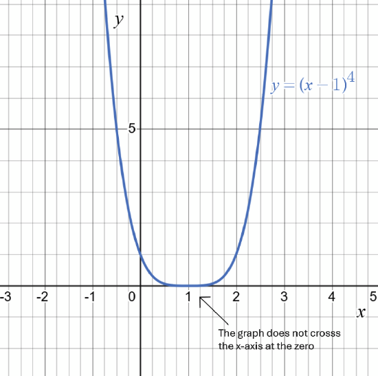
If the zero $x=1$ has multiplicity four, then a possible formula is $y=(x-1)^4$. The graph is a shift right one of the even power $y=x^4$ which does not cross the x-axis at the zero as shown in the graph below.

$the graph of a fourth degree power function that does not cross the x-axis at the zero.$

If the zero $x=1$ has multiplicity five, then a possible formula is $y=(x-1)^5$. The graph is a shift right one of the odd power $y=x^5$. So the graph will cross the x-axis at the zero as shown in the graph below.

$The graph of a 5th degree power that crosses the x-axis at its zero.$

In general, a polynomial function with a single real zero with odd multiplicity will have a graph that is a horizontal shift of an odd power which will cross the x-axis at the zero (with or without a vertical stretch or reflection of the graph). A polynomial function with a single real zero with even multiplicity will have a graph that is a horizontal shift of an even power which will not cross the x-axis at the zero.

Key Point $\PageIndex{3}$

The graph of a polynomial function with a real zero $x=k$ with odd multiplicity will cross the x-axis at the zero. The graph of a polynomial function with a real zero $x=k$ with even multiplicity will not cross the x-axis at the zero.

Case: The effect of other distinct zeros near a zero.

Consider the polynomial $y=x^3(x-1)$ where the zero $x=1$ has multiplicity one. Notice that as $x$ nears the zero $x=1$ from above, the factor (x-1) nears 0, the factor $x^3$ nears 1, so the product $y=x^3(x-1)$ nears $0 \cdot 1 = 0$ as illustrated in the table below.

The effect of mutiple factors on the function value near a zero.
$x$	2	1.5	1.1	1.001	1.0001
$x-1$	1	0.5	0.1	0.001	0.0001
$x^3$	8	3.375	1.331	1.003	1.0003
$y=x^3(x-1)$	8	1.686	0.1331	0.001	0.0001

Moreover, the other factor $x^3$ does not change sign near the zero $x=1$, but the factor $ (x-1) $ does change sign near the zero $x=1$ since it has odd multiplicity. Therefore, the product $y=x^3(x-1)$ will change sign at the zero. A similar table with values of $x$ approaching $x=1$ from below will yield a similar result. Therefore, we can conclude the multiplicity of a real zero, determines the behavior of the graph near that real zero. The other factor(s) and corresponding zeros do not effect the behavior of the graph near a specific zero.

Now we are ready to graph polynomials.

Focus: Graphing Polynomials

With the zeros of a polynomial, their multiplicity, and the end behavior, we have enough key features to sketch a graph of a polynomial.

Example $\PageIndex{3}$

Let $f(x) = x^3 - 4x^2+4x $.

Identify the zeros and their multiplicities.
Determine whether the graph crosses the x-axis at each zero.
Determine the end behavior.
Use the zeros, their multiplicity, and the end behavior to graph the polynomial $f(x)$.

Solution

Factoring the polynomial, we have \[f(x) = x^3 - 4x^2+4x = x(x^2-4x+4) = x(x-2)(x-2) \nonumber \] The factors correspond to the zero $x=0$ with multiplicity one and the zero $x=2$ with multiplicity two.
Since the zero $x=0$ has odd multiplicity, the graph will cross the x-axis at $x=0$. Since the zero $x=2$ has even multiplicity, the graph will not cross the x-axis at $x=2$.
The end behavior of $f(x)$ resembles the end behavior of the term of largest power $y=x^3$. Therefore, the end behavior resembles that of an odd power with no reflection $ (a=1) $ which opens up on the right (as $x \to \infty$, $y \to \infty$) and down on the left (as $x \to \infty$, $y \to \infty$).
From the rightmost zero at $x=2$, the graph opens upward to the right due to the right end behavior. The graph can't cross the x-axis for any $x>2$ otherwise their would be a third distinct zero, a contradiction since their are only two real zeros. From the leftmost zero at $x=0$, the graph opens downward to the left due to the left end behavior. As we move from the left to right along the graph, the graph crosses the x-axis at zero $x=0$, then must change direction, before dropping down to the x-axis at the other zero $x=2$. Since this zero has even multiplicity, the graph does not cross the x-axis at this zero.

$the graph of a cubic polynomial that crosses the x-axis at x=0 and touches but does not cross at x=2.$

Example $\PageIndex{4}$

Let $f(x) = x^4 - x^3+6x^2 $.

Identify the zeros and their multiplicities.
Determine whether the graph crosses the x-axis at each zero.
Determine the end behavior.
Use the zeros, their multiplicity, and the end behavior to graph the polynomial $f(x)$.

Solution

Factoring the polynomial, we have \[f(x) = x^4 - x^3-6x^2 = x^2(x^2-x-6) = x^2(x-3)(x+2) \nonumber \] The factors correspond to the zero are $x=0$ with multiplicity two, the zero $x=3$ with multiplicity one, and the zero $x=-2$ with multiplicity one.
Since the zero $x=0$ has even multiplicity, the graph will not cross the x-axis at $x=0$. Since the zeros $x=3$ and $x=-2 $ have odd multiplicity, the graph will cross the x-axis at these zeros.
The end behavior of $f(x)$ resembles the end behavior of the term of largest power $y=x^4$. Therefore, the end behavior resembles that of an even power with no reflection $ (a=1) $ which opens upward on both ends (as $x \to \pm \infty$, $y \to \infty$ ).
From the rightmost zero at $x=3$, the graph opens upward to the right due to the right end behavior. Using the same rational as example 4.3.3, the graph can't cross the x-axis for any $x>3$ otherwise their would be a fourth zero, a contradiction since their are only three distinct real zeros. From the leftmost zero at $x=-2$, the graph opens upward to the left due to the left end behavior. As we move from the left to right along the graph, the graph crosses the x-axis at zero $x=-2$, then must change direction, and come up to the x-axis at the next zero $x=0$. Since the zero $x=0$ has even multiplicity, the graph does not cross the x-axis at this zero. Continuing rightward along the graph, the graph decreases, then must change direction, and come up to the x-axis at the next zero $x=3$. The graph crosses the x-axis at the zero $x=3$.

$the graph of a polynomial with x-intercepts at x=0, x = 3, and x = -2.$

Example $\PageIndex{5}$

Let $f(x) = x^3 - 13x+12 $.

Identify the zeros and their multiplicities.
Determine the end behavior.
Use the zeros, their multiplicity, and the end behavior to graph the polynomial $f(x)$.

Solution

Since their is no common factor, we must use the rational zero theorem to identify a rational zero if one exists. The possible zeros are $x= \dfrac{\pm 1, \pm 2, \pm 3, \pm 4, \pm 6, \pm 12}{\pm 1} $. In example 4.2.9, we tested a number of possible zeros for $f(x)$ before we determined that $x=1$ was a zero since $ f(1)=0 $. In example 4.2.1, we divided $f(x) = x^3 - 13x+12$ by the corresponding factor $(x-1)$ of the zero $x=1$ using long division of polynomials. We found that \[\dfrac{x^3 - 13x+12}{x-1}=x^2+x-12 \nonumber \]This allowed us to factor $f(x)$ as \[f(x) = x^3 - 13x+12 = (x-1)(x^2+x-12) = (x-1)(x-3)(x+4) \nonumber \] The factors correspond to zeros of $x=1$, $x=3$, and $x=-4$ aeach with multiplicity one. The graph will cross the x-axis at these zeros due to their multiplicities.
The end behavior of $f(x)$ resembles the end behavior of the term of largest power $y=x^3$. Therefore, the end behavior resembles that of an odd power with no reflection $ (a=1)$ which opens upward on the right end (as $x \to \infty$, $y \to \infty$ ) and downward on the left end (as $x \to -\infty$, $y \to -\infty$ ).
From the rightmost zero at $x=3$, the graph opens upward to the right due to the right end behavior. From the leftmost zero at $x=-4$, the graph opens downward to the left due to the left end behavior. As we move from the left to right along the graph, the graph crosses the x-axis at zero $x=-4$, then must change direction and come back down to the x-axis at the next zero $x=1$ where it crosses the x-axis. Continuing rightward along the graph, the graph continues to decreas, then must change direction and come up to the x-axis at the next zero at $x=3$ where it crosses the x-axis.

$The graph of a polynomial function that crosses the x-axis at the zeros x= -4, x= 1, and x = 3.$

We can also use the graph of a polynomial to determine its formula, now that we can identify the multiplicity based on the behavior of the graph at each real zero.

Example $\PageIndex{6}$

Identify a possible formula for the graph of the polynomial given below that passes through the point (1,8).

$the graph of a polynomial function that passes through the point (-1,8) with x-intercepts at x=-2, x = 0, and x = 1.$

Solution

The x-intercepts at $x=-2$, $x=0$, and $x=1$ are the real zeros of the polynomials. Since the graph crosses the x-axis at the zero $x=-2$, the zero has odd multiplicity and therefore the polynomial has an odd number of factors of the corresponding factor $(x+2)$. Since the graph does not cross the x-axis at the zero $x=0$, the zero has even multiplicity and therefore the polynomial has an even number of factors of the corresponding factor $(x)$. Since the graph does not cross the x-axis at the zero $x=1$, the zero has even multiplicity and the polynomial has an even number of factors of the corresponding factor $(x-1)$. So a possible formula of minimum degree would be \[f(x)= ax^2(x+2)(x-1)^2 \nonumber\] To find the stretch factor $a$, we can substitute the known point $x=-1$ and $y=8$ into the polynomial \[a(-1)^2(-1+2)(-1-1)^2=8 \nonumber \] Then solving for $a$, we have \[a4=8 \nonumber \] \[a=2 \nonumber \] Therefore, the formula for the polynomial is \[f(x)= 2x^2(x+2)(x-1)^2 \nonumber\]

Now You Try: Exercise $\PageIndex{3}$

Let $f(x) = -2x^4 + 4x^3+6x^2 $.

Identify the zeros and their multiplicities.
Determine whether the graph crosses the x-axis at each zero.
Determine the end behavior.
UUse the zeros, their multiplicity, and the end behavior to graph the polynomial $f(x)$.

Answer

The zeros are $x=0$ with multiplicity two, $x=3$ with multiplicity one, and $x=-1$ with multiplicity one.
The graph will not cross the x-axis at $x=0$ since it has even multiplicity. The graph will cross the x-axis at the zeros $x=3$ and $x=-1$ since they have odd multiplicity.
The end behavior resembles that of a reflection of an even power which opens downward on both ends (as $x \to \pm \infty$, $y \to -\infty$ ).
$The graph of a polynomial function that crosses the x-axis at the zeros x = -1 and x = 3. The graph touches the x-axis at x= 0 but does not cross.$

Now You Try: Exercise $\PageIndex{4}$

The graph of a polynomial function $y=f(x)$ containing the point (0,1.8) is given below.

Identify each real zero and its smallest possible multiplicity.
Write a formula for the polynomial function. Assume the least polynomial is of least possible degree.

$The graph of a polynomial that crosses the x-axis at x = -1. The graph does not cross the x-axis at the x-intercepts x = -3 and x = 1.$

Answer: $y=f(x)=0.2(x+3)^2(x+1)(x-1)^2 $

Important Topics of this Section

The End Behavior of Polynomial Functions
The Effect of The Multiplicity of A Zero on the Graph
Graphing Polynomials

Search

Text Color

Text Size

Margin Size

Font Type

Key Point \(\PageIndex{1}\): The End Behavior of Powers of \(x\)

Key Point \(\PageIndex{2}\): The Effect of The Stretch Factor on The End Behavior

Example \(\PageIndex{1}\)

Solution

Now You Try: Exercise \(\PageIndex{1}\)

Key Point \(\PageIndex{3}\): The End Behavior of a Polynomial

Example \(\PageIndex{2}\)

Solution

Now You Try: Exercise \(\PageIndex{2}\)

Key Point \(\PageIndex{2}\)

Key Point \(\PageIndex{3}\)

Example \(\PageIndex{3}\)

Solution

Example \(\PageIndex{4}\)

Solution

Example \(\PageIndex{5}\)

Solution

Example \(\PageIndex{6}\)

Solution

Now You Try: Exercise \(\PageIndex{3}\)

Now You Try: Exercise \(\PageIndex{4}\)

\(x\)	\(x^2\)	\(x^3\)	\(x^3+x^2\)	The percent of \(x^3\) as a portion of the total value of the polynomial \(x^3+x^2\)
1	1	1	2	\(\dfrac{1}{2} = 0.5 \) = 50%
10	100	1,000	1,100	\(\dfrac{1,000}{1,100} \approx 0.9091 \) = 90.91%
100	10,000	1,000,000	1,010,000	\(\dfrac{1,000,000}{1,010,000} \approx 0.990099 \) = 99.0099%
1000	1,000,000	1,000,000,000	1,001,000,000	\(\dfrac{1,000,000,000}{1,001,000,000} \approx 0.999 \) = 99.9%

\(x\)	2	1.5	1.1	1.001	1.0001
\(x-1\)	1	0.5	0.1	0.001	0.0001
\(x^3\)	8	3.375	1.331	1.003	1.0003
\(y=x^3(x-1)\)	8	1.686	0.1331	0.001	0.0001