1.10: The Derivative as a Function

Learning Objectives Define the derivative function of a given function. Graph a derivative function from the graph of a given function. State the connection between derivatives and continuity. Describe three conditions when a function has no derivative. Explain the meaning of a higher-order derivative.

Hawk A.I. Section-Specific Tutor Please note that, to access the Hawk A.I. Tutor, you will need a (free) OpenAI account.

As we have seen, the derivative of a function at a given point gives us the rate of change or slope of the tangent line to the function at that point. We obtain the velocity if we differentiate a position function at a given time. Knowing the function's derivative at every point produces valuable information about the function's behavior. However, finding the derivative at even a handful of values using the techniques of the preceding section would quickly become quite tedious. In this section, we define the derivative function and learn a process for finding it.

Derivative Functions

The derivative function gives the derivative of a function at each point in the domain of the original function for which the derivative is defined. We can formally define a derivative function as follows.

Definition: Derivative Function

Let $f$ be a function. The derivative function, denoted by $f^{\prime}$, is the function whose domain consists of those values of $x$ such that the following limit exists: $$f^{\prime}(x)=\lim_{h \to 0}\dfrac{f(x+h)−f(x)}{h}. \label{derdef}$$

A function $f(x)$ is said to be differentiable at $a$ if $f^{\prime}(a)$ exists. More generally, a function is said to be differentiable on $S$ if it is differentiable at every point in an open set $S$, and a differentiable function is one in which $f^{\prime}(x)$ exists on its domain.

In the next few examples we use Equation $\ref{derdef}$ to find the derivative of a function.

Example $\PageIndex{1}$: Finding the Derivative of a Square-Root Function

Find the derivative of $f(x)=\sqrt{x}$.

Solution

Start directly with the definition of the derivative function.

Substitute $f(x+h)=\sqrt{x+h}$ and $f(x)=\sqrt{x}$ into $f^{\prime}(x)= \displaystyle \lim_{h \to 0}\frac{f(x+h)−f(x)}{h}$. $$\begin{array}{rcl} f^{\prime}(x) & = & \displaystyle \lim_{h \to 0}\dfrac{\sqrt{x+h}−\sqrt{x}}{h} \\[16pt] & = & \displaystyle\lim_{h \to 0}\dfrac{\left( \sqrt{x+h}−\sqrt{x} \right)}{h} \cdot \dfrac{\left( \sqrt{x+h}+\sqrt{x} \right)}{\left( \sqrt{x+h}+\sqrt{x} \right)} \\[16pt] & = & \displaystyle\lim_{h \to 0}\dfrac{h}{h\left(\sqrt{x+h}+\sqrt{x}\right)} \\[16pt] & = & \displaystyle\lim_{h \to 0}\dfrac{\cancelto{1}{h}}{\cancel{h}\left(\sqrt{x+h}+\sqrt{x}\right)} \\[16pt] & = & \displaystyle\lim_{h \to 0}\dfrac{1}{\sqrt{x+h}+\sqrt{x}} \\[16pt] & \overset{\text{D.S.}}{=} & \dfrac{1}{2\sqrt{x}} \\ \end{array} \nonumber$$

Example $\PageIndex{2}$: Finding the Derivative of a Quadratic Function

Find the derivative of the function $f(x)=x^2−2x$.

Solution

Follow the same procedure, but without multiplying by the conjugate.

Substitute $f(x+h)=(x+h)^2−2(x+h)$ and $f(x)=x^2−2x$ into $f^{\prime}(x)= \displaystyle \lim_{h \to 0}\frac{f(x+h)−f(x)}{h}$. $$\begin{array}{rcl} f^{\prime}(x) & = & \displaystyle \lim_{h \to 0}\dfrac{((x+h)^2−2(x+h))−(x^2−2x)}{h} \\[16pt] & = & \displaystyle\lim_{h \to 0}\dfrac{x^2+2xh+h^2−2x−2h−x^2+2x}{h} \\[16pt] & = & \displaystyle\lim_{h \to 0}\dfrac{2xh−2h+h^2}{h} \\[16pt] & = & \displaystyle\lim_{h \to 0}\dfrac{h(2x−2+h)}{h} \\[16pt] & = & \displaystyle\lim_{h \to 0}\dfrac{\cancelto{1}{h}(2x−2+h)}{\cancelto{1}{h}} \\[16pt] & = & \displaystyle\lim_{h \to 0}(2x−2+h) \\[16pt] & \overset{\text{D.S.}}{=} & 2x−2 \\ \end{array} \nonumber$$

Checkpoint $\PageIndex{2}$

Find the derivative of $f(x)=x^2$.

Answer

$f^{\prime}(x)=2x$

Notations for the Derivative

There is no single uniform notation for differentiation. Instead, various notations for the derivative of a function or variable have been proposed by various mathematicians. The usefulness of each notation varies with the context, and it is sometimes advantageous to use more than one notation in a given context.

Lagrange's Notation: $f^{\prime}(x)$

One of the most common modern notations for differentiation is named after Joseph Louis Lagrange, even though Euler invented it and Lagrange just popularized it. In Lagrange's notation, a prime mark denotes a derivative. If $y = f(x)$ is a function, then its derivative evaluated at $x$ is written $$\displaystyle f^{\prime}(x) \quad \text{(a common alternative form is } y^{\prime} \text{)} \nonumber$$ Lagrange's notation first appeared in print in 1749.

If the derivative is evaluated at $x =a$, then the value is written as $f^{\prime}(a)$ or $y^{\prime}(a)$.

Leibniz's Notation: $\dfrac{dy}{dx}$

The original notation employed by Gottfried Leibniz is still frequently used throughout mathematics. It is prevalent when the equation $y = f(x)$ is regarded as a functional relationship between dependent and independent variables $y$ and $x$. Leibniz's notation makes this relationship explicit by writing the derivative as $$\displaystyle \dfrac{dy}{dx} \quad \left(\text{common alternative forms are }\dfrac{df(x)}{dx}, \dfrac{df}{dx}(x), \text{ and } \dfrac{d}{dx}f(x) \right) \nonumber$$ In Example $\PageIndex{2}$, we could have expressed the derivative as $\frac{dy}{dx}=2x−2$. We could have conveyed the same information by writing $\frac{d}{dx}\left(x^2−2x\right)=2x−2$.

To understand this notation better, recall that the derivative of a function at a point is the limit of the slopes of secant lines as the secant lines approach the tangent line. The slopes of these secant lines are often expressed in the form $\frac{ \Delta y}{ \Delta x}$ where $\Delta y$ is the difference in the $y$ values corresponding to the difference in the $x$ values, which are expressed as $\Delta x$ (Figure $\PageIndex{1}$). Thus the derivative, which can be thought of as the instantaneous rate of change of $y$ with respect to $x$, is expressed as $$\displaystyle \dfrac{dy}{dx}= \lim_{ \Delta x \to 0}\dfrac{ \Delta y}{ \Delta x}.\nonumber$$

Figure $\PageIndex{1}$: The derivative is expressed as $\frac{dy}{dx}=\displaystyle\lim_{ \Delta x \to 0}\frac{ \Delta y}{ \Delta x}$.

If the derivative is evaluated at $x = a$, then the value is written as $\frac{dy}{dx}\Big|_{x = a}$ or $\frac{df}{dx}\Big|_{x = a}$.

Caution: Careful Use of Leibniz's Notation

When using Leibniz's notation to find the derivative of $y = f(x)$ at $x = a$, it is incorrect to write $\frac{df(a)}{dx}$. The reason for this will be explored in the next chapter.

Euler's Notation: $D$

Leonhard Euler's notation uses a differential operator suggested by Louis François Antoine Arbogast, denoted as $D$. When applied to a function $f(x)$, it is defined by $$(Df)(x) \nonumber$$ Euler's notation is useful in a subject called differential equations; however, we will not be using it in this text.

Newton's Notation: $\dot{y}$

Isaac Newton's notation for differentiation (also called the dot notation, fluxions, or sometimes, crudely, the flyspeck notation for differentiation) places a dot over the dependent variable. That is if $y$ is a function of $t$, then the derivative of $y$ with respect to $t$ is $$\dot{y} \nonumber$$ This notation is popular in physics and mathematical physics. It also appears in areas of mathematics connected with physics, such as differential equations. As with Euler's notation, we will not be using Newton's notation in this text.

Graphing a Derivative

We have already discussed how to graph a function, so given the equation of a function or the equation of a derivative function, we could graph it. Given both, we would expect to see a correspondence between the graphs of these two functions since $f^{\prime}(x)$ gives the rate of change of a function $f(x)$ (or slope of the tangent line to $f(x)$).

In Example $\PageIndex{1}$, we found that for $f(x)=\sqrt{x}$, $f^{\prime}(x)=\frac{1}{2\sqrt{x}}$. If we graph these functions on the same axes, as in Figure $\PageIndex{2}$, we can use the graphs to understand the relationship between these two functions. First, we notice that $f(x)$ is increasing over its entire domain, which means that the slopes of its tangent lines at all points are positive. Consequently, we expect $f^{\prime}(x)>0$ for all values of $x$ in its domain. Furthermore, as $x$ increases, the slopes of the tangent lines to $f(x)$ are decreasing. We expect to see a corresponding decrease in $f^{\prime}(x)$. We also observe that $f(0)$ is undefined and that $\displaystyle \lim_{x \to 0^+}f^{\prime}(x)=+\infty$, corresponding to a vertical tangent to $f(x)$ at $0$.

Figure $\PageIndex{2}$: The derivative $f^{\prime}(x)$ is positive everywhere because the function $f(x)$ is increasing.

In Example $\PageIndex{2}$, we found that for $f(x)=x^2−2x,\; f^{\prime}(x)=2x−2$. The graphs of these functions are shown in Figure $\PageIndex{3}$. Observe that $f(x)$ is decreasing for $x<1$. For these same values of $x$, $f^{\prime}(x)<0$. For values of $x>1$, $f(x)$ is increasing and $f^{\prime}(x)>0$. Also, $f(x)$ has a horizontal tangent at $x=1$ and $f^{\prime}(1)=0$.

Figure $\PageIndex{3}$: The derivative $f^{\prime}(x)<0$ where the function $f(x)$ is decreasing and $f^{\prime}(x)>0$ where $f(x)$ is increasing. The derivative is zero where the function has a horizontal tangent

Example $\PageIndex{3}$: Sketching a Derivative Using a Function

Use the following graph of $f(x)$ to sketch a graph of $f^{\prime}(x)$.

Solution

The solution is shown in the following graph. Observe that $f(x)$ is increasing and $f^{\prime}(x)>0$ on $(–2,3)$. Also, $f(x)$ is decreasing and $f^{\prime}(x)<0$ on $(−\infty,−2)$ and on $(3,+\infty)$. Also note that $f(x)$ has horizontal tangents at $–2$ and $3$, and $f^{\prime}(−2)=0$ and $f^{\prime}(3)=0$.

Checkpoint $\PageIndex{3}$

Sketch the graph of $f(x)=x^2−4$. On what interval is the graph of $f^{\prime}(x)$ above the $x$-axis?

Answer

$(0,+\infty)$

Derivatives and Continuity

Now that we can graph a derivative let's examine the behavior of the graphs. First, we consider the relationship between differentiability and continuity. We will see that if a function is differentiable at a point, it must be continuous there; however, a continuous function need not be differentiable at that point. A function may be continuous at a point and fail to be differentiable at the point for one of several reasons.

Theorem: Differentiability Implies Continuity

Let $f(x)$ be a function and $a$ be in its domain. If $f(x)$ is differentiable at $a$, then $f$ is continuous at $a$.

Proof

If $f(x)$ is differentiable at $a$, then $f^{\prime}(a)$ exists and, if we let $h = x - a$, we have $x = a + h$, and as $h=x-a\to 0$, we can see that $x\to a$.

Then $$f^{\prime}(a) = \lim_{h\to 0}\dfrac{f(a+h)-f(a)}{h}\nonumber$$ can be rewritten as $$f^{\prime}(a)=\displaystyle \lim_{x \to a}\dfrac{f(x)−f(a)}{x−a}.\nonumber$$ We want to show that $f(x)$ is continuous at $a$ by showing that $\displaystyle \lim_{x \to a}f(x)=f(a).$ Thus, $$\begin{array}{rcl} \displaystyle \lim_{x \to a}f(x) & = & \displaystyle \lim_{x \to a}\;\big(f(x)−f(a)+f(a)\big) \\[16pt] & = & \displaystyle \lim_{x \to a}\left(\dfrac{f(x)−f(a)}{x−a} \cdot (x−a)+f(a)\right) \\[16pt] & = & \left(\displaystyle \lim_{x \to a}\dfrac{f(x)−f(a)}{x−a}\right) \cdot \left( \displaystyle \lim_{x \to a}\;(x−a)\right)+\displaystyle \lim_{x \to a} f(a) \\[16pt] & = & f^{\prime}(a) \cdot 0+f(a) \\[16pt] & = & f(a). \\ \end{array}\nonumber$$ Therefore, since $f(a)$ is defined and $\displaystyle \lim_{x \to a}f(x)=f(a)$, we conclude that $f$ is continuous at $a$.

Q.E.D.

We have just proven that differentiability implies continuity, but now we consider whether continuity implies differentiability. To determine an answer to this question, we examine the function $f(x)=|x|$. This function is continuous everywhere; however, $f^{\prime}(0)$ is undefined. This observation leads us to believe that continuity does not imply differentiability. Let's explore further. For $f(x)=|x|$, $$f^{\prime}(0)=\displaystyle \lim_{x \to 0}\dfrac{f(x)−f(0)}{x−0}= \lim_{x \to 0}\dfrac{|x|−|0|}{x−0}= \lim_{x \to 0}\dfrac{|x|}{x}.\nonumber$$ This limit does not exist because $$\displaystyle \lim_{x \to 0^−}\dfrac{|x|}{x}=−1 \quad \text{and} \quad \displaystyle \lim_{x \to 0^+}\dfrac{|x|}{x}=1.\nonumber$$ See Figure $\PageIndex{4}$.

Figure $\PageIndex{4}$: The function $f(x)=|x|$ is continuous at $0$ but is not differentiable at $0$.

Let's consider some additional situations in which a continuous function fails to be differentiable. Consider the function $f(x)=\sqrt[3]{x}$: $$f^{\prime}(0)=\displaystyle \lim_{x \to 0}\dfrac{\sqrt[3]{x}−0}{x−0}=\displaystyle \lim_{x \to 0}\dfrac{1}{\sqrt[3]{x^2}}=+\infty.\nonumber$$ Thus $f^{\prime}(0)$ does not exist. A quick look at the graph of $f(x)=\sqrt[3]{x}$ clarifies the situation. The function has a vertical tangent line at $0$ (Figure $\PageIndex{5}$).

Figure $\PageIndex{5}$: The function $f(x)=\sqrt[3]{x}$ has a vertical tangent at $x=0$. It is continuous at $0$ but is not differentiable at $0$.

The function $f(x)=\begin{cases} x\sin\left(\frac{1}{x}\right), & & \text{ if } x \neq 0\\0, & & \text{ if } x=0\end{cases}$ also has a derivative that exhibits interesting behavior at $0$.

We see that $$f^{\prime}(0)=\displaystyle \lim_{x \to 0}\dfrac{x\sin\left(1/x\right)−0}{x−0}= \lim_{x \to 0}\sin\left(\dfrac{1}{x}\right).\nonumber$$ This limit does not exist, essentially because the slopes of the secant lines continuously change direction as they approach zero (Figure $\PageIndex{6}$).

Figure $\PageIndex{6}$: The function $f(x)=\begin{cases} x\sin\left(\frac{1}{x}\right), & & \text{ if } x \neq 0\\0, & & \text{ if } x=0\end{cases}$ is not differentiable at $0$.

In summary:

• We observe that if a function is not continuous, it cannot be differentiable since every differentiable function must be continuous. However, if a function is continuous, it may still fail to be differentiable.
• We saw that $f(x)=|x|$ failed to be differentiable at $0$ because the limits of the slopes of the tangent lines on the left and right were not the same. Visually, this resulted in a sharp corner on the function's graph at $0.$. From this, we conclude that to be differentiable at a point, a function must be "smooth" at that point.
• As we saw in the example of $f(x)=\sqrt[3]{x}$, a function fails to be differentiable at a point where there is a vertical tangent line.
• As we saw with $f(x)=\begin{cases}x\sin\left(\frac{1}{x}\right), & & \text{ if } x \neq 0\\0, & &\text{ if } x=0\end{cases}$ a function may fail to be differentiable at a point in more complicated ways as well.

Example $\PageIndex{4}$: A Piecewise Function that is Continuous and Differentiable

A toy company wants to design a track for a toy car that starts along a parabolic curve and then converts to a straight line (Figure $\PageIndex{7}$). The function that describes the track is to have the form $f(x)=\begin{cases}\frac{1}{10}x^2+bx+c, & & \text{ if }x<−10\\−\frac{1}{4}x+\frac{5}{2}, & & \text{ if } x \geq −10\end{cases}$ where $x$ and $f(x)$ are in inches. For the car to move smoothly along the track, the function $f(x)$ must be both continuous and differentiable at $−10$. Find values of $b$ and $c$ that make $f(x)$ both continuous and differentiable.

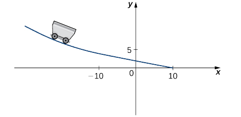
Figure $\PageIndex{7}$: The function must be continuous and differentiable for the car to move smoothly along the track.

Solution

For the function to be continuous at $x=−10$, $\displaystyle \lim_{x \to 10^−}f(x)=f(−10)$. Thus, since $$\displaystyle \lim_{x \to −10^−}f(x)=\dfrac{1}{10}(−10)^2−10b+c=10−10b+c\nonumber$$ and $f(−10)=5$, we must have $10−10b+c=5$. Equivalently, we have $c=10b−5$.

For the function to be differentiable at $−10$, $$f^{\prime}(10)=\displaystyle \lim_{x \to −10}\dfrac{f(x)−f(−10)}{x+10}\nonumber$$ must exist. Since $f(x)$ is defined using different rules on the right and the left, we must evaluate this limit from the right and the left and then set them equal to each other: $$\begin{array}{rcl} \displaystyle \lim_{x \to −10^−}\dfrac{f(x)−f(−10)}{x+10} & = & \displaystyle \lim_{x \to −10^−}\dfrac{\frac{1}{10}x^2+bx+c−5}{x+10} \\[16pt] & = & \displaystyle \lim_{x \to −10^−}\dfrac{\frac{1}{10}x^2+bx+(10b−5)−5}{x+10} \\[16pt] & = & \displaystyle \lim_{x \to −10^−}\dfrac{x^2−100+10bx+100b}{10(x+10)} \\[16pt] & = & \displaystyle \lim_{x \to −10^−}\dfrac{(x+10)(x−10+10b)}{10(x+10)} \\[16pt] & = & b−2 \\ \end{array}\nonumber$$ We also have $$\begin{array}{rcl} \displaystyle \lim_{x \to −10^+}\dfrac{f(x)−f(−10)}{x+10} & = & \displaystyle \lim_{x \to −10^+}\dfrac{−\frac{1}{4}x+\frac{5}{2}−5}{x+10} \\[16pt] & = & \displaystyle \lim_{x \to −10^+}\dfrac{−(x+10)}{4(x+10)} \\[16pt] & = & −\dfrac{1}{4} \\ \end{array} \nonumber$$ This gives us $b−2=−\frac{1}{4}$. Thus $b=\frac{7}{4}$ and $c=10(\frac{7}{4})−5=\frac{25}{2}$.

Checkpoint $\PageIndex{4}$

Find values of a and b that make $f(x)=\begin{cases}ax+b, & & \text{ if } x<3\\x^2, & & \text{ if } x \geq 3\end{cases}$ both continuous and differentiable at $3$.

Answer

$a=6$ and $b=−9$

Higher-Order Derivatives

The derivative of a function is itself a function, so we can find the derivative of a derivative. For example, the derivative of a position function is the rate of change of position or velocity. The derivative of velocity is the rate of change of velocity, which is acceleration. The new function obtained by differentiating the derivative is called the second derivative. Furthermore, we can continue taking derivatives to obtain the third, fourth, and so on. Collectively, these are referred to as higher-order derivatives. The notation for the higher-order derivatives of $y=f(x)$ can be expressed in any of the following forms: $$\begin{array}{c} f^{\prime\prime}(x),\; f^{\prime\prime\prime}(x),\; f^{(4)}(x),\; \ldots \; ,\; f^{(n)}(x) \\ y^{\prime\prime}(x),\; y^{\prime\prime\prime}(x),\; y^{(4)}(x),\; \ldots \; ,\; y^{(n)}(x) \\ \dfrac{d^2y}{dx^2},\;\dfrac{d^3y}{dy^3},\;\dfrac{d^4y}{dy^4},\; \ldots \;,\;\dfrac{d^ny}{dy^n}. \\ \end{array} \nonumber$$ It is interesting to note that the notation for $\frac{d^2y}{dx^2}$ may be viewed as an attempt to express $\frac{d}{dx}\left(\frac{dy}{dx}\right)$ more compactly.

Analogously, $\frac{d}{dx}\left(\frac{d}{dx}\left(\frac{dy}{dx}\right)\right)=\frac{d}{dx}\left(\frac{d^2y}{dx^2}\right)=\frac{d^3y}{dx^3}$.

Example $\PageIndex{5}$: Finding a Second Derivative

For $f(x)=2x^2−3x+1$, find $f^{\prime\prime}(x)$.

Solution

First find $f^{\prime}(x)$.

Substitute $f(x)=2x^2−3x+1$ and $f(x+h)=2(x+h)^2−3(x+h)+1$ into $f^{\prime}(x)=\displaystyle \lim_{h \to 0}\frac{f(x+h)−f(x)}{h}$. $$\begin{array}{rcl} f^{\prime}(x) & = & \displaystyle \lim_{h \to 0}\dfrac{(2(x+h)^2−3(x+h)+1)−(2x^2−3x+1)}{h} \\[16pt] & = & \displaystyle \lim_{h \to 0}\dfrac{4xh+2h^2−3h}{h} \\[16pt] & = & \displaystyle \lim_{h \to 0}(4x+2h−3) \\[16pt] & \overset{\text{D.S.}}{=} & 4x−3 \\ \end{array} \nonumber$$ Next, find $f^{\prime\prime}(x)$ by taking the derivative of $f^{\prime}(x)=4x−3$. $$\begin{array}{rcl} f^{\prime\prime}(x) & = & \displaystyle \lim_{h \to 0}\dfrac{f^{\prime}(x+h)−f^{\prime}(x)}{h} \\[16pt] & = & \displaystyle \lim_{h \to 0}\dfrac{(4(x+h)−3)−(4x−3)}{h} \\[16pt] & = & \displaystyle \lim_{h \to 0}4 \\[16pt] & \overset{\text{D.S.}}{=} & 4 \\ \end{array} \nonumber$$

Checkpoint $\PageIndex{5}$

Find $f^{\prime\prime}(x)$ for $f(x)=x^2$.

Answer

$f^{\prime\prime}(x)=2$

Example $\PageIndex{6}$: Finding Acceleration

The position of a particle along a coordinate axis at time $t$ (in seconds) is given by $s(t)=3t^2−4t+1$ (in meters). Find the function that describes its acceleration at time $t$.

Solution

Since $v(t)=s^{\prime}(t)$ and $a(t)=v^{\prime}(t)=s^{\prime\prime}(t)$, we begin by finding the derivative of $s(t)$: $$\begin{array}{rcl} s^{\prime}(t) & = & \displaystyle \lim_{h \to 0}\dfrac{s(t+h)−s(t)}{h} \\[16pt] & = & \displaystyle \lim_{h \to 0}\dfrac{3(t+h)^2−4(t+h)+1−(3t^2−4t+1)}{h} \\[16pt] & = & 6t−4 \\ \end{array}\nonumber$$ Next, $$\begin{array}{rcl} s^{\prime\prime}(t) & = & \displaystyle \lim_{h \to 0}\dfrac{s^{\prime}(t+h)−s^{\prime}(t)}{h} \\[16pt] & = & \displaystyle \lim_{h \to 0}\dfrac{6(t+h)−4−(6t−4)}{h} \\[16pt] & = & 6 \\ \end{array}\nonumber$$ Thus, $a=6 \;\text{m/s}^2$.

Checkpoint $\PageIndex{6}$

For $s(t)=t^3$, find $a(t).$

Answer

$a(t)=6t$