1.7: Hyperbolic Functions

Hanging cables form a curve called a catenary. These curves are modeled using a new (to you) family of functions called the hyperbolic functions.

Learning Objectives

• Identify the hyperbolic functions, their graphs, and basic identities.

Unlike all the material in this chapter up to this point, the material in the section should be unfamiliar to you. In this section we define hyperbolic and inverse hyperbolic functions, which involve combinations of exponential and logarithmic functions. These provide a unique bridge between two groups of transcendental functions - exponential and trigonometric.

---

From Circular to Hyperbolic Functions

Before we introduce the hyperbolic functions, it is worthwhile to investigate a particular feature of the trigonometric functions.

Most people refer to the sine, cosine, tangent, and their reciprocals as the trigonometric functions; however, they are also known as circular functions. This is because their entire definition is based on the unit circle. Recall, the unit circle is defined by the relation

\[ x^2 + y^2 = 1. \nonumber \]

The graph of this relation can be seen in Figure \( \PageIndex{1} \) below.

Figure \( \PageIndex{1} \): The unit circle.

During our journey through Trigonometry, we discovered that the length of the arc on the unit circle subtended by an angle \( \theta \) (in radians) is \( s = \theta \). Moreover, we derived the area of a sector formula to be

\[ A = \dfrac{1}{2} r^2 \theta. \nonumber \]

Since the radius of the unit circle is \( r=1 \) and \( \theta = s \), we arrived at the fact that the area seen in Figure \( \PageIndex{2} \) is

\[ A = \dfrac{s}{2}. \nonumber \]

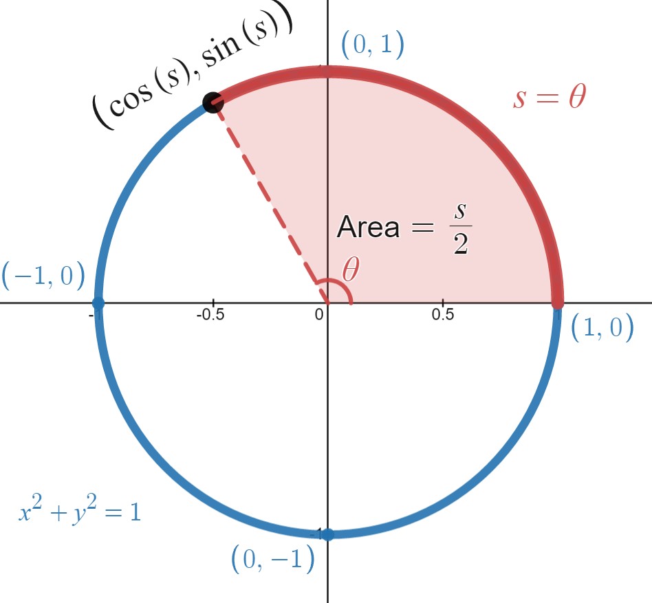
Figure \( \PageIndex{2} \): The area of the sector of the unit circle having arc length \( s \) is \( \frac{s}{2} \).

Stated clearly, the area of the region bounded by

1. the positive \( x \)-axis,
2. the unit circle, and
3. the line segment connecting the origin to the point \( (\cos{(s)}, \sin{(s)}) \)

is \( s/2 \).

In this section we ask the following question:

Could we develop a set of functions, let's call them \( \cosh{(s)} \) and \( \sinh{(s)} \), such that the area of the region bounded by

1. the positive \( x \)-axis,
2. the unit hyperbola, and
3. the line segment connecting the origin to the point \( (\cosh{(s)} , \sinh{(s)}) \)

is \( s/2 \)?

Before we can answer this question, we need to define the unit hyperbola. For our purposes, the unit hyperbola will be defined by the relation

\[ x^2 - y^2 = 1. \nonumber \]

Furthermore, we restrict our work to the right branch of this hyperbola (see Figure \( \PageIndex{3} \)).

Figure \( \PageIndex{3} \): The unit hyperbola (right branch only).

We plot a point \( (x,y) = (\cosh{(s)} , \sinh{(s)})\) on this branch, highlight the arc length along the unit hyperbola to this point, draw a line segment connecting the origin to this point, and shade the bounded region (see Figure \( \PageIndex{4} \)).

Figure \( \PageIndex{4} \): We desire \( \cosh{(s)} \) and \( \sinh{(s)} \) so that the shaded region is \( s/2 \).

We want to define these new functions, \( \cosh{(s)} \) and \( \sinh{(s)} \), so that the shaded region is \( s/2 \).

Caution

It is critical to point out here that the highlighted arc length will not be \( s \). In fact, the angle between the positive \( x \)-axis and the line segment connecting the origin to the point \( (\cosh{(s)}, \sinh{(s)}) \) will also not be \( s \). Our goal with this discussion is not to find the arc length nor to find the angle, but instead to create functions, \( \cosh{(s)} \) and \( \sinh{(s)} \), so that the area of the bounded region is \( s/2 \).

As you can see in Figure \( \PageIndex{4} \), we define the hyperbolic cosine to be the \( x \)-value of this terminal point, and the hyperbolic sine as the \( y \)-value. We denote these functions as \( \cosh{(s)} \) and \( \sinh{(s)} \), respectively.

---

Hyperbolic Functions

The previous discussion considered the hyperbolic cosine and hyperbolic sine as functions of \( s \); however, most textbooks work exclusively with these as functions of \( t \). Since \( s \) is a "dummy variable," we can replace it easily with \( t \) for the remainder of this section.

It turns out (and can be proven in Calculus II) that the hyperbolic cosine and the hyperbolic sine can be written in terms of certain combinations of \(e^t\) and \(e^{−t}\). These functions arise naturally in various engineering and physics applications, including the study of water waves and vibrations of elastic membranes. Another common use, at least for the hyperbolic cosine, is the representation of a hanging chain or cable, also known as a catenary (Figure \(\PageIndex{5}\)). If we introduce a coordinate system so that the low point of the chain lies along the \(y\)-axis, we can describe the height of the chain in terms of the hyperbolic cosine.

Figure \(\PageIndex{5}\):The shape of a strand of silk in a spider’s web can be described in terms of a hyperbolic function. The same shape applies to a chain or cable hanging from two supports with only its own weight. (credit: “Mtpaley”, Wikimedia Commons)

Theorem: Hyperbolic Functions

Let \( \frac{t}{2} \) be the area of the region bounded by the arc along the right branch of the unit hyperbola \( x^2 - y^2 = 1 \) whose initial point is \( \left( 1,0 \right) \) and terminal point is \( \left( x,y \right) \), the \( x \)-axis, and the line segment connecting the origin to \( \left( x, y \right) \). Then the hyperbolic functions in terms of twice this bounded area, are defined (and derived) as follows:¹

Hyperbolic cosine

\(x = \cosh{(t)} = \dfrac{e^t+e^{−t}}{2}\)

Hyperbolic sine

\(y = \sinh{(t)} = \dfrac{e^t−e^{−t}}{2}\)

Hyperbolic tangent

\(\tanh{(t)} = \dfrac{\sinh{(t)}}{\cosh{(t)}} = \dfrac{e^t−e^{−t}}{e^t+e^{−t}}\)

Hyperbolic cosecant

\(\operatorname{csch}{(t)} = \dfrac{1}{\sinh{(t)}} = \dfrac{2}{e^t−e^{−t}}\)

Hyperbolic secant

\(\operatorname{sech}{(t)} = \dfrac{1}{\cosh{(t)}} = \dfrac{2}{e^t+e^{−t}}\)

Hyperbolic cotangent

\(\coth{(t)} = \dfrac{\cosh{(t)}}{\sinh{(t)}} = \dfrac{e^t+e^{−t}}{e^t−e^{−t}}\)

We have not proven that the hyperbolic functions are equal to these exponential forms despite writing this as a theorem. The reality is that you need Integral Calculus (Calculus II) to prove these relationships.

The name \(\cosh\) rhymes with "gosh," whereas the name \(\sinh\) is pronounced "sinch." \(\operatorname{Tanh}, \,\operatorname{sech}, \, \operatorname{csch},\) and \(\coth\) are pronounced "tanch," "seech," "coseech," and "cotanch," respectively.

Example \(\PageIndex{1}\): Evaluating Hyperbolic Functions

Simplify \(\sinh{ \left( 5\ln{(x)} \right) } \).

Solution

Using the definition of the \(\sinh\) function, we get

\[ \begin{array}{rclcr}
\sinh{ \left( 5\ln{(x)} \right) } & = & \dfrac{e^{5\ln{(x)}} − e^{−5\ln{(x)}}}{2} & & \left( \text{Calculus: Definition of Hyperbolic Functions} \right) \\
 & = & \dfrac{e^{\ln{(x^5)}} − e^{\ln{(x^{-5})}}}{2} & & \left( \text{Algebra: Laws of Logarithms} \right) \\
 & = & \dfrac{x^5 − x^{-5}}{2} & & \left( \text{Algebra: Exponentials and logarithms are inverses} \right) \\
\end{array} \nonumber \]

Exercise \(\PageIndex{1}\)

Simplify \(\cosh(2\ln x)\).

Hint

Use the definition of the \(\cosh\) function and the power property of logarithm functions.

Answer

\((x^2+x^{−2})/2\)

Subsection Footnotes

¹ The \( x \)-value of the terminal point along the unit hyperbola is defined to be \( \cosh{(t)} \) and the \( y \)-value is defined to be \( \sinh{(t)} \). The exponential forms, \[ \cosh{(t)} = \dfrac{e^t+e^{−t}}{2} \text{ and } \sinh{(t)} = \dfrac{e^t−e^{−t}}{2} \nonumber \] are derived using techniques in Calculus II. The remaining hyperbolic functions are defined as ratios of the \( \sinh{(t)} \) and \( \cosh{(t)} \).

---

Graphs of Hyperbolic Functions

To investigate the graphs of the hyperbolic functions, we need to start with a discussion related to Calculus - what happens to \( e^{-x} \) as \( x \to \infty \)? At this very early point in Differential Calculus, it's best to build a table of values to investigate this behavior (although, tables of values to investigate such behavior will be highly frowned upon as we move forward in Calculus).

Table \( \PageIndex{1} \): Exploring \( e^{-x} \) as \( x \to \infty \)

\( x \)	\( 1 \)	\( 10 \)	\( 100 \)	\( 1000 \)
\( e^{-x} \)	\( 0.3678794412 \)	\( 4.53999298 \times 10^{-5} \)	\( 3.72007598 \times 10^{-44} \)	too small for Desmos

It seems like \( e^{-x} \to 0 \) as \( x \to \infty \). A similar exploration shows the possibility that \( e^x \to 0 \) as \( x \to -\infty \).² Therefore,

\[ \sinh{(x)} = \dfrac{e^x - e^{-x}}{2} \to \dfrac{e^x}{2}, \text{ as }x \to \infty, \text{ and } \cosh{(x)} = \dfrac{e^x + e^{-x}}{2} \to \dfrac{e^x}{2}, \text{ as }x \to \infty \nonumber \]

Likewise,

\[ \sinh{(x)} = \dfrac{e^x - e^{-x}}{2} \to \dfrac{-e^{-x}}{2}, \text{ as }x \to -\infty, \text{ and } \cosh{(x)} = \dfrac{e^x + e^{-x}}{2} \to \dfrac{e^{-x}}{2}, \text{ as }x \to -\infty \nonumber \]

Hence, using the graphs of \(\frac{1}{2}e^x\), \(\frac{1}{2}e^{−x}\), and \(−\frac{1}{2}e^{−x}\) as guides, we can graph \(\cosh(x)\) and \(\sinh(x)\).

To graph \(\tanh(x)\), we use the fact that \(\tanh(0)=0\) along with the fact that the numerator is smaller (in magnitude) than the denominator (as can be seen from the exponential form of \( \tanh{(x)} \). Therefore, \(−1<\tanh(x)<1\) for all \(x\). A quick investigation demonstrates the possibility that \(\tanh(x) \to 1\) as \(x \to \infty\), and \(\tanh(x) \to −1\) as \(x \to −\infty\). The graphs of the other three hyperbolic functions can be sketched using the graphs of \(\cosh(x)\), \(\sinh(x)\), and \(\tanh(x)\) (Figure \(\PageIndex{6}\)).³

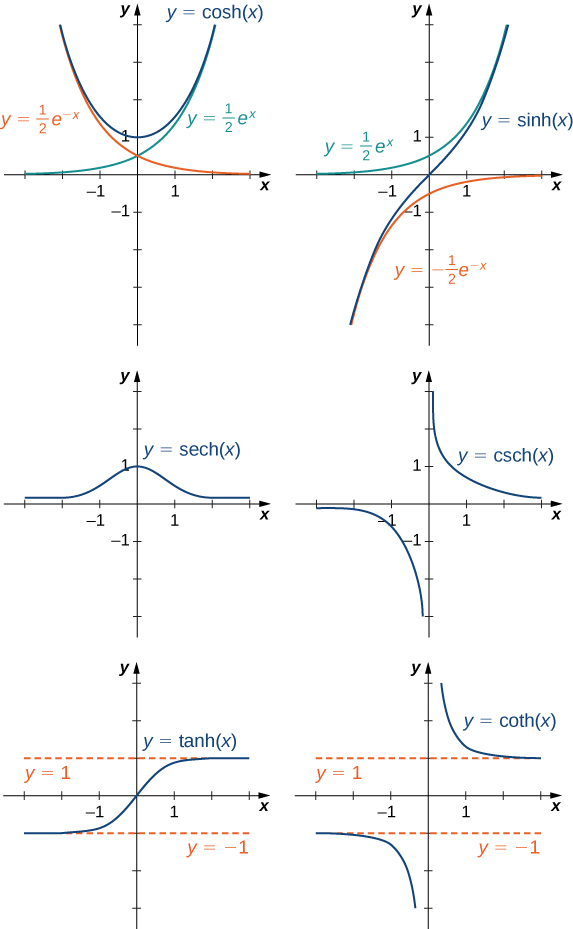
Figure \(\PageIndex{6}\): The hyperbolic functions involve combinations of \(e^x\) and \(e^{−x}\).

Subsection Footnotes

² I am trying to be very careful with my wording here. A calculator can only demonstrate possible behavior (as we will investigate in Chapter 2); however, we need to use Calculus to prove that observation is true before we can be certain.

³ While you will be expected to know the basic shapes of the graphs of \( \cosh{(x)} \) and \( \sinh{(x)} \). The graphs of the remaining four hyperbolic functions are rarely used in practice.

---

Hyperbolic Identities

Once you grasp that the hyperbolic functions are based on the unit hyperbola, \( x^2 - y^2 = 1 \), you immediately arrive at the first of many hyperbolic identities.

Theorem: The Fundamental Hyperbolic Identity

\[ \cosh^2{(t)} - \sinh^2{(t)} = 1 \nonumber \]

Proof

Since \( x = \cosh{(t)} \) and \( y = \sinh{(t)} \) on the unit hyperbola \( x^2 - y^2 = 1 \), we substitute to arrive at \( \cosh^2{(t)} - \sinh^2{(t)} = 1\).

It is also important to note that this can be proved using the exponential form of the hyperbolic functions.

The Fundamental Hyperbolic Identity is one of many identities involving the hyperbolic functions, some of which are listed next.⁴ The first four properties follow easily from the definitions of hyperbolic sine and hyperbolic cosine. Except for some differences in signs, most of these properties are analogous to identities for trigonometric functions.

Theorem: Basic Hyperbolic Identities

1. \(\cosh(−t)=\cosh(t)\)
2. \(\sinh(−t)=−\sinh(t)\)
3. \(\cosh(t)+\sinh(t) = e^t\)
4. \(\cosh(t) −\sinh(t) = e^{−t}\)
5. \(1−\tanh^2(t) = \operatorname{sech}^2(t)\)
6. \(\coth^2(t) −1=\operatorname{csch}^2(t) \)
7. \(\sinh(t \pm v)=\sinh(t) \cosh(v) \pm \cosh(t) \sinh(v)\)
8. \(\cosh(t \pm v)=\cosh(t) \cosh(v) \pm \sinh(t) \sinh(v)\)

Example \(\PageIndex{2}\): Evaluating Hyperbolic Functions

If \(\sinh{(t)} = 3/4\), find the values of the remaining five hyperbolic functions.

Solution

Using the identity \(\cosh^2{(t)} − \sinh^2{(t)} = 1\),we see that

\[ \cosh^2{(t)} = 1 + \left(\frac{3}{4}\right)^2 = \dfrac{25}{16}. \nonumber \]

Since \(\cosh x \geq 1\) for all \(x\), we must have \(\cosh x=5/4\). Then, using the definitions for the other hyperbolic functions, we conclude that \(\tanh x=3/5,\operatorname{csch}x=4/3,\operatorname{sech}x=4/5\), and \(\coth x=5/3\).

Example \(\PageIndex{3}\): Proving a Hyperbolic Identity

Without using \(\cosh(t \pm v)=\cosh(t) \cosh(v) \pm \sinh(t) \sinh(v)\), prove

\[ \cosh{(2t)} = \sinh^2{(t)} + \cosh^2{(t)}. \nonumber \]

Solution

\[ \begin{array}{rclcr}
\cosh^2{(t)} + \sinh^2{(t)} & = & \left( \dfrac{e^{t} + e^{-t}}{2} \right)^2 + \left( \dfrac{e^{t} - e^{-t}}{2} \right)^2 & \quad & \left( \text{Calculus: Exponential form of hyperbolic functions} \right) \\
 & = & \dfrac{e^{2t} + 2 + e^{-2t}}{4} + \dfrac{e^{2t} - 2 + e^{-2t}}{4} & \quad & \left( \text{Algebra: Squaring binomials and Laws of Exponents} \right) \\
 & = & \dfrac{2 e^{2t} + 2 e^{-2t}}{4} & \quad & \left( \text{Algebra: Combining like terms} \right) \\
 & = & \dfrac{\cancel{2} \left(e^{2t} + e^{-2t}\right)}{\cancel{2} \cdot 2} & \quad & \left( \text{Algebra: Factor out the GCF and cancel like factors} \right) \\
 & = & \dfrac{e^{2t} + e^{-2t}}{2} & \quad & \left( \text{Algebra: Cancel like factors} \right) \\
 & = & \cosh{(2t)} & \quad & \left( \text{Calculus: Exponential form of hyperbolic functions} \right) \\
\end{array} \nonumber \]

Subsection Footnotes

⁴ As with identities encountered in Trigonometry, the number of identities involving hyperbolic functions is too numerous to contain within a single table.

---

Inverse Hyperbolic Functions

From the graphs of the hyperbolic functions, we see that all of them are one-to-one except \(\cosh x\) and \(\operatorname{sech}x\). If we restrict the domains of these two functions to the interval \([0,\infty),\) then all the hyperbolic functions are one-to-one, and we can define the inverse hyperbolic functions. Since the hyperbolic functions themselves involve exponential functions, it should make sense to the reader that the inverse hyperbolic functions involve logarithmic functions.

Theorem: Inverse Hyperbolic Functions

\[\begin{align*} &\sinh^{−1}x =\operatorname{arcsinh}x=\ln \left(x+\sqrt{x^2+1}\right) & & \cosh^{−1}x =\operatorname{arccosh}x=\ln \left(x+\sqrt{x^2−1}\right)\\[4pt]
&\tanh^{−1}x=\operatorname{arctanh}x=\dfrac{1}{2}\ln \left(\dfrac{1+x}{1−x}\right) & & \coth^{−1}x =\operatorname{arccot}x=\frac{1}{2}\ln \left(\dfrac{x+1}{x−1}\right)\\[4pt]
&\operatorname{sech}^{−1}x=\operatorname{arcsech}x=\ln \left(\dfrac{1+\sqrt{1−x^2}}{x}\right) & & \operatorname{csch}^{−1}x=\operatorname{arccsch}x=\ln \left(\dfrac{1}{x}+\dfrac{\sqrt{1+x^2}}{|x|}\right) \end{align*}\]

Proof that \( \sinh^{−1}x =\ln \left(x+\sqrt{x^2+1}\right) \)

Suppose \(y=\sinh^{−1}x\). Then, \(x=\sinh y\) and, by the definition of the hyperbolic sine function, \(x=\dfrac{e^y−e^{−y}}{2}\). Therefore,

\(e^y−2x−e^{−y}=0.\)

Multiplying this equation by \(e^y\), we obtain

\(e^{2y}−2xe^y−1=0\).

This can be solved like a quadratic equation, with the solution

\(e^y=\dfrac{2x \pm \sqrt{4x^2+4}}{2}=x \pm \sqrt{x^2+1}\).

Since \(e^y>0\),the only solution is the one with the positive sign. Applying the natural logarithm to both sides of the equation, we conclude that

\(y=\ln (x+\sqrt{x^2+1}).\)

Q.E.D.

Caution

The independent variable \( x \) in the previous theorem is a dummy variable. It is not the \( x \)-coordinate of the terminal point of the arc of length \( t \) along the unit hyperbola.

Example \(\PageIndex{4}\): Evaluating Inverse Hyperbolic Functions

Evaluate each of the following expressions.

\(\sinh^{−1}(2)\)

\(\tanh^{−1}(1/4)\)

Solution

\[\sinh^{−1}(2)=\ln (2+\sqrt{2^2+1})=\ln (2+\sqrt{5}) \approx 1.4436\nonumber \]

\[\tanh^{−1}(1/4)=\frac{1}{2}\ln \left(\dfrac{1+1/4}{1−1/4}\right)=\frac{1}{2}\ln \left(\dfrac{5/4}{3/4}\right)=\frac{1}{2}\ln \left(\dfrac{5}{3}\right) \approx 0.2554\nonumber \]

Exercise \(\PageIndex{4}\)

Evaluate \(\tanh^{−1}(1/2)\).

Hint

Use the definition of \(\tanh^{−1}x\) and simplify.

Answer

\(\dfrac{1}{2}\ln (3) \approx 0.5493\).

---

Key Concepts

• The hyperbolic functions involve combinations of the exponential functions \(e^x\) and \(e^{−x}.\) As a result, the inverse hyperbolic functions involve the natural logarithm.

---

Glossary

hyperbolic functions

the functions denoted \(\sinh,\,\cosh,\,\operatorname{tanh},\,\operatorname{csch},\,\operatorname{sech},\) and \(\coth\), which involve certain combinations of \(e^x\) and \(e^{−x}\)

inverse hyperbolic functions

the inverses of the hyperbolic functions where \(\cosh\) and \( \operatorname{sech}\) are restricted to the domain \([0,\infty)\);each of these functions can be expressed in terms of a composition of the natural logarithm function and an algebraic function