1.8: Moments and Centers of Mass

Learning Objectives

• Determine the mass of a one-dimensional object from its linear density function.
• Determine the mass of a two-dimensional circular object from its radial density function.
• Find the center of mass of objects distributed along a line.
• Locate the center of mass of a thin plate.
• Use symmetry to help locate the centroid of a thin plate.
• Apply the theorem of Pappus for volume.

In this section, we consider centers of mass (also called centroids, under certain conditions) and moments. The basic idea of the center of mass is a balancing point. Many of us have seen performers spin plates on the ends of sticks. The performers try to keep several spinning without allowing them to drop. If we look at a single plate (without spinning it), there is a sweet spot where it balances perfectly on the stick. If we put the stick anywhere other than that sweet spot, the plate does not balance and falls to the ground. (That is why performers spin the plates; the spin helps keep the plates from falling even if the stick is not exactly in the right place.) Mathematically, that sweet spot is called the center of mass of the plate.

This section examines these concepts in a one-dimensional context. Then, we expand our development to consider centers of mass of two-dimensional regions and symmetry. Last, we use centroids to find the volume of certain solids by applying the Theorem of Pappus.

Mass and Linear Density

We can use integration to develop a formula for calculating mass based on a linear density function. First, we consider a thin rod or wire. Orient the rod so it aligns with the $x$-axis, with the left end of the rod at $x=a$ and the right end of the rod at $x=b$ (Figure $\PageIndex{1}$). Note that although we depict the rod with some thickness in the figures, for mathematical purposes, we assume the rod is thin enough to be treated as a one-dimensional object.

Figure $\PageIndex{1}$: We can calculate the mass of a thin rod oriented along the $x$-axis by integrating its linear density function.

If the rod has constant linear density $\rho$, given in terms of mass per unit length (i.e., $\rho = m/\mathcal{l}$), then the mass of the rod is just the product of the linear density and the length of the rod. That is, $$m = \rho (b - a). \nonumber$$ If the linear density of the rod is not constant, however, the problem becomes a little more challenging. When the linear density of the rod varies from point to point, we use a linear density function, $\rho(x)$, to denote the density of the rod at any point, $x$. Let $\rho(x)$ be an integrable linear density function. Now, for $i=0,1,2, \ldots ,n$ let $P=\{x_i\}$ be a regular partition of the interval $[a,b]$, and for $i=1,2, \ldots ,n$ choose an arbitrary point $x^∗_i \in [x_{i−1},x_i]$. Figure $\PageIndex{2}$ shows a representative segment of the rod.

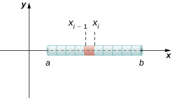
Figure $\PageIndex{2}$: A representative segment of the rod.

The mass, $m_i$, of the segment of the rod from $x_{i−1}$ to $x_i$ is approximated by $$\begin{array}{rcl} m_i & \approx & \rho(x^∗_i)(x_i−x_{i−1}) \\ & = & \rho(x^∗_i) \Delta x. \\ \end{array} \nonumber$$ Adding the masses of all the segments gives us an approximation for the mass of the entire rod: $$\begin{array}{rcl} m & = & \displaystyle \sum_{i=1}^n m_i \\[12pt] & \approx & \displaystyle \sum_{i=1}^n\rho(x^∗_i) \Delta x. \\ \end{array} \nonumber$$ This is a Riemann sum. Taking the limit as $n \to \infty$, we get an expression for the exact mass of the rod: $$\begin{array}{rcl} m & = & \displaystyle \lim_{n \to \infty }\sum_{i=1}^n\rho(x^∗_i) \Delta x \\[12pt] & = & \displaystyle \int ^b_a \rho(x) \,dx. \\ \end{array} \nonumber$$ We state this result in the following theorem.

Theorem: Mass–Linear Density and Weight-Linear Weight Density Formulas of a One-Dimensional Object

Given a thin rod oriented along the $x$-axis over the interval $[a,b]$, let $\rho(x)$ denote a linear density function giving the density of the rod at a point $x$ in the interval. Then the mass of the rod is given by $$m=\int ^b_a \rho(x) \, dx. \label{density1}$$ If given the linear weight density function, $\gamma(x)$, then the weight of the rod is given by $$F = \int_a^b \gamma(x) \, dx. \label{weight1}$$

Before we move on, we must understand how the units work with Equations $\ref{density1}$ and $\ref{weight1}$.

In Equation $\ref{density1}$, we are given the linear density function $\rho(x)$. The unit types for this density function are $$\dfrac{\text{mass}}{\text{length}}, \nonumber$$ where the mass unit could be in kilograms, grams, slugs, or any other unit of mass we are interested in, and the length unit is in meters, centimeters, feet, inches, or whatever unit of length in which we are interested. The unit type for $dx$ is length (which we would make sure matches the units of the length in the density function). Hence, the unit type for the integral is $$\dfrac{\text{mass}}{\cancelto1{\text{length}}} \cdot \cancelto1{\text{length}} = \text{mass}, \nonumber$$ which is exactly what we are trying to compute.

Likewise, in Equation $\ref{weight1}$, we are given the linear weight density function $\gamma(x)$. The unit types for this weight density function are $$\dfrac{\text{force}}{\text{length}}, \nonumber$$ where the force unit could be either in pounds or newtons (and only those two choices), and the length unit is in meters, centimeters, feet, inches, or whatever unit of length in which we are interested. The unit type for $dx$ is length (which we would make sure matches the units of the length in the weight density function). Hence, the unit type for the integral is $$\dfrac{\text{force}}{\cancelto1{\text{length}}} \cdot \cancelto1{\text{length}} = \text{force}, \nonumber$$ which is, again, exactly what we are trying to compute.

The previous discussion using unit analysis will be especially helpful in physics and engineering (and, luckily, the homework). We apply this theorem in the next example.

Example $\PageIndex{1}$: Calculating Mass from Linear Density

Consider a thin rod oriented on the $x$-axis over the interval $\left[ \frac{\pi}{2}, \pi \right]$. If the linear density of the rod is given by $\rho(x)=\sin x$, what is the mass of the rod?

Solution

Applying Equation $\ref{density1}$ directly, we have $$\begin{array}{rcl} m & = & \displaystyle \int ^b_a\rho(x) \, dx \\[12pt] & = & \displaystyle \int ^ \pi _{ \pi /2}\sin x \,dx \\[12pt] & = & -\cos x \Big|^ \pi _{ \pi /2} \\[12pt] & = & 1. \\ \end{array} \nonumber$$

Checkpoint $\PageIndex{1}$

Consider a thin rod oriented on the $x$-axis over the interval $[1,3]$. If the linear density of the rod is given by $\rho(x)=2x^2+3,$ what is the mass of the rod?

Answer

$70/3$

Mass and Radial Density

We now extend this concept to find the mass of a two-dimensional disk of radius $r$. As with the rod we looked at in the one-dimensional case, here we assume the disk is thin enough that, for mathematical purposes, we can treat it as a two-dimensional object. We assume the density is given in terms of mass per unit area (i.e., $\rho = m/A$), which is why this is often called the area density. For this discussion, we will further assume the area density varies only along the disk's radius. In this situation, we could call the area density by a different name - the radial density. This is because it is a function of how far away a point is from the disk's center.

We orient the disk in the $xy$-plane, with the center at the origin. Then, the density of the disk can be treated as a function of $x$, denoted $\rho(x)$. We assume $\rho(x)$ is integrable. Because density is a function of $x$, we partition the interval from $[0,r]$ along the $x$-axis. For $i=0,1,2, \ldots ,n$, let $P=\{x_i\}$ be a regular partition of the interval $[0,r]$, and for $i=1,2, \ldots ,n$, choose an arbitrary point $x^∗_i \in [x_{i−1},x_i]$. Use the partition to break the disk into thin (two-dimensional) washers. A disk and a representative washer are depicted in the following figure.

Figure $\PageIndex{3a}$: A thin disk in the $xy$-plane.
Figure $\PageIndex{ 3b }$: A representative washer.

We now approximate the density and area of the washer to calculate an approximate mass, $m_i$. Note that the area of the washer is given by $$\begin{array}{rcl} A_i & = & \pi (x_i)^2− \pi (x_{i−1})^2 \\ & = & \pi [x^2_i−x^2_{i−1}] \\ & = & \pi (x_i+x_{i−1})(x_i−x_{i−1}) \\ & = & \pi (x_i+x_{i−1}) \Delta x. \\ \end{array} \nonumber$$ You may recall that we had an expression similar to this when we were computing volumes by the Method of Cylindrical Shells. As we did there, we use $x^∗_i \approx (x_i+x_{i−1})/2$ to approximate the average radius of the washer. We obtain $$A_i = \pi (x_i+x_{i−1}) \Delta x \approx 2 \pi x^∗_i \Delta x. \nonumber$$ Using $\rho(x^∗_i)$ to approximate the (radial) density of the washer, we approximate the mass of the washer by $$m_i \approx 2 \pi x^∗_i\rho(x^∗_i) \Delta x. \nonumber$$ Adding up the masses of the washers, we see the mass $m$ of the entire disk is approximated by $$m = \sum_{i=1}^n m_i \approx \sum_{i=1}^n2 \pi x^∗_i\rho(x^∗_i) \Delta x. \nonumber$$ We again recognize this as a Riemann sum and take the limit as $n \to \infty .$ This gives us $$\begin{array}{rcl} m & = & \displaystyle \lim_{n \to \infty }\sum_{i=1}^n 2 \pi x^∗_i\rho(x^∗_i) \Delta x \\[12pt] & = & \displaystyle \int ^r_0 2 \pi x \rho(x) \, dx. \\ \end{array} \nonumber$$ We summarize these findings in the following theorem.

Theorem: Mass–Radial Density and Weight-Radial Weight Density Formulas of a Circular Object

Let $\rho(x)$ be an integrable function representing the radial density of a disk of radius $r$. Then the disk's mass is given by $$m=\int ^r_0 2 \pi x\rho(x) \, dx. \label{massEq1}$$ If given the radial weight density function, $\gamma(x)$, the weight of the disk is given by $$F = \int^r_0 2 \pi x \gamma(x) \, dx. \label{weightEq1}$$

As we did with linear density, a unit analysis discussion for radial density is helpful.

In Equation $\ref{massEq1}$, we are given the radial density function $\rho(x)$. The unit types for this radial density function are $$\dfrac{\text{mass}}{\text{length}^2}, \nonumber$$ where, just like before, the mass unit could be in kilograms, grams, slugs, or any other unit of mass we are interested in, and the length unit is in meters, centimeters, feet, inches, or whatever unit of length in which we are interested. The unit type for $dx$ is length, and the unit type for $x$ is also length. Hence, the unit type for the integral is $$\text{length} \cdot \dfrac{\text{mass}}{\text{length}^2} \cdot \text{length} = \dfrac{\text{mass}}{\cancelto1{\text{length}^2}} \cdot \cancelto1{\text{length}^2} = \text{mass}, \nonumber$$ which is exactly what we are trying to compute.

Likewise, in Equation $\ref{weightEq1}$, we are given the radial weight density function $\gamma(x)$. The unit types for this radial weight density function are $$\dfrac{\text{force}}{\text{length}^2}, \nonumber$$ where, yet again, the force unit could be either in pounds or newtons. The length unit is in meters, centimeters, feet, inches, or whatever unit of length we are interested in. The unit type for $dx$ is length, and the unit type for $x$ is also length. Hence, the unit type for the integral is $$\text{length} \cdot \dfrac{\text{force}}{\text{length}^2} \cdot \text{length} = \dfrac{\text{force}}{\cancelto1{\text{length}^2}} \cdot \cancelto1{\text{length}^2} = \text{force}, \nonumber$$ which is, again, exactly what we are trying to compute.

Example $\PageIndex{2}$: Calculating Mass from Radial Density

Let $\rho(x)=\sqrt{x}$ represent the radial density of a disk. Calculate the mass of a disk of radius 4.

Solution

Applying Equation $\ref{massEq1}$, we find $$\begin{array}{rcl} m & = & \displaystyle \int ^r_0 2 \pi x\rho(x) \, dx \\[12pt] & = & \displaystyle \int ^4_0 2 \pi x\sqrt{x} \, dx \\[12pt] & = & 2 \pi \displaystyle \int ^4_0 x^{3/2} \, dx \\[12pt] & = & \dfrac{4 \pi}{5}x^{5/2}\bigg|^4_0 \\[12pt] & = & \dfrac{128 \pi }{5}. \\ \end{array} \nonumber$$

Checkpoint $\PageIndex{2}$

Let $\rho(x)=3x+2$ represent the radial density of a disk. Calculate the mass of a disk of radius 2.

Answer

$24 \pi$

Center of Mass and Moments

Media

• Moments and Centers of Mass for Discrete Point-Masses

We now step away from standard shapes like rods and circles and instead try to focus on irregular-shaped regions. Specifically, we want to discuss a given two-dimensional object's center of mass (the balancing point). To do so, however, we first need a bit of theory.

Let's begin by looking at the center of mass in a one-dimensional context. Consider a long, thin wire or rod of negligible mass resting on a fulcrum, as shown in Figure $\PageIndex{4a}$. Now suppose we place objects having masses $m_1$ and $m_2$ at distances $d_1$ and $d_2$ from the fulcrum, respectively, as shown in Figure $\PageIndex{4b}$.

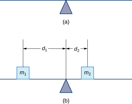
Figure $\PageIndex{4a}$: A thin rod rests on a fulcrum.
Figure $\PageIndex{ 4b }$: Masses are placed on the rod.

The most common real-life example of a system like this is a playground seesaw, or teeter-totter, with children of different weights sitting at different distances from the center. On a seesaw, if one child sits at each end, the heavier child sinks, and the lighter child is lifted into the air. Suppose the heavier child slides in toward the center, though the seesaw balances. Applying this concept to the masses on the rod, we note that the masses balance each other if and only if $$m_1 d_1 = m_2 d_2. \nonumber$$ In the seesaw example, we balanced the system by moving the masses (children) with respect to the fulcrum. However, we are interested in systems where the masses cannot move. Instead, we balance the system by moving the fulcrum. Suppose we have two point masses,¹ $m_1$ and $m_2$, located on a number line at points $x_1$ and $x_2$, respectively (Figure $\PageIndex{5}$). The center of mass, $\bar{x}$, is where the fulcrum should be placed to balance the system.

Figure $\PageIndex{5}$: The center of mass $\bar{x}$ is the balance point of the system.

Thus, we have $$\begin{array}{rrcl} & m_1 |x_1−\bar{x}| & = & m_2|x_2−\bar{x}| \\ \implies & m_1(\bar{x}−x_1) & = & m_2(x_2−\bar{x}) \\ \implies & m_1\bar{x}−m_1x_1 & = & m_2x_2−m_2\bar{x} \\ \implies & \bar{x}(m_1+m_2) & = & m_1x_1+m_2x_2 \\ \end{array} \nonumber$$ or $$\bar{x} =\dfrac{m_1x_1+m_2x_2}{m_1+m_2} \label{COM}$$ The expression in the numerator of Equation $\ref{COM}$, $m_1x_1+m_2x_2$, is called the first moment of the system with respect to the origin. If the context is clear, we often drop the word first and refer to this expression as the moment of the system. The expression in the denominator, $m_1+m_2$, is the system's total mass. Thus, the center of mass of the system is the point at which the system's total mass could be concentrated without changing the moment.

This idea is more expansive than two point masses. In general, if $n$ masses, $m_1,m_2, \ldots ,m_n$, are placed on a number line at points $x_1,x_2, \ldots ,x_n$, respectively, then the center of mass of the system is given by $$\bar{x}=\dfrac{ {\sum_{i=1}^nm_ix_i}}{ {\sum_{i=1}^nm_i}}. \nonumber$$

Theorem: Center of Mass of Objects on a Line

Let $m_1,m_2, \ldots ,m_n$ be point masses placed on a number line at points $x_1,x_2, \ldots ,x_n$, respectively, and let $m= \displaystyle \sum_{i=1}^n m_i$ denote the total mass of the system. Then, the moment of the system with respect to the origin is given by $$M=\sum_{i=1}^n m_i x_i \label{moment}$$ and the center of mass of the system is given by $$\bar{x}=\dfrac{M}{m}. \label{COM2a}$$

We apply this theorem in the following example.

Example $\PageIndex{3}$: Finding the Center of Mass of Objects along a Line

Suppose four point masses are placed on a number line as follows:

• $m_1 = 30\, \text{kg},$ placed at $x_1=−2\, \text{m}$
• $m_2=5\, \text{kg},$ placed at $x_2=3\, \text{m}$
• $m_3=10\, \text{kg},$ placed at $x_3=6\, \text{m}$
• $m_4=15\, \text{kg},$ placed at $x_4=−3\, \text{m.}$

Find the moment of the system with respect to the origin and find the center of mass of the system.

Solution

First, we need to calculate the moment of the system (Equation $\ref{moment}$): $$\begin{array}{rcl} M & = & \displaystyle \sum_{i=1}^4 m_i x_i \\[12pt] & = & −60+15+60−45 \\[12pt] & = & −30. \\ \end{array} \nonumber$$ Now, to find the center of mass, we need the total mass of the system: $$\begin{array}{rcl} m & = & \displaystyle \sum_{i=1}^4 m_i \\[12pt] & = & 30+5+10+15 \\[12pt] & = & 60\, \text{kg} \\ \end{array} \nonumber$$ Then we have (from Equation $\ref{COM2a}$) $$\bar{x} = \dfrac{M}{m} = −\dfrac{30}{60} = −\dfrac{1}{2}. \nonumber$$ The center of mass is located 1/2 m to the left of the origin.

Checkpoint $\PageIndex{3}$

Suppose four point masses are placed on a number line as follows:

• $m_1=12\, \text{kg}$ placed at $x_1=−4\, \text{m}$
• $m_2=12\, \text{kg}$ placed at $x_2=4\, \text{m}$
• $m_3=30\, \text{kg}$ placed at $x_3=2\, \text{m}$
• $m_4=6\, \text{kg},$ placed at $x_4=−6\, \text{m.}$

Find the moment of the system with respect to the origin and find the center of mass of the system.

Answer

$M=24,\bar{x}=\frac{2}{5}\, \text{m}$

We can generalize this concept to find the center of mass of a system of point masses in a plane.

Let $m_1$ be a point mass located at point $(x_1,y_1)$ in the plane. Then the moment $M_x$ of the mass with respect to the $x$-axis is given by $M_x = m_1 y_1$. Similarly, the moment $M_y$ with respect to the $y$-axis is given by $M_y = m_1 x_1$.

Notice that the $x$-coordinate of the point is used to calculate the moment with respect to the $y$-axis, and vice versa. The reason is that the $x$-coordinate gives the distance from the point mass to the $y$-axis, and the $y$-coordinate gives the distance to the $x$-axis (see Figure $\PageIndex{6}$).

Figure $\PageIndex{6}$: Point mass $m_1$ is located at point $(x_1,y_1)$ in the plane.

If we have several point masses in the $xy$-plane, we can use the moments with respect to the $x$- and $y$-axes to calculate the $x$- and $y$-coordinates of the center of mass of the system.

Theorem: Center of Mass of Objects in a Plane

Let $m_1, m_2, \ldots , m_n$ be point masses located in the $xy$-plane at points $(x_1,y_1),(x_2,y_2), \ldots ,(x_n,y_n)$, respectively, and let $m = \displaystyle \sum_{i=1}^n m_i$ denote the total mass of the system. Then the moments $M_x$ and $M_y$ of the system with respect to the $x$- and $y$-axes, respectively, are given by $$M_x = \sum_{i=1}^n m_i y_i \label{COM1}$$ and $$M_y = \sum_{i=1}^n m_i x_i. \label{COM2}$$ Also, the coordinates of the center of mass $(\bar{x},\bar{y})$ of the system are $$\bar{x} = \dfrac{M_y}{m} \label{COM3}$$ and $$\bar{y}=\dfrac{M_x}{m}. \label{COM4}$$

The next example demonstrates how the center of mass formulas (Equations $\ref{COM1}$ - $\ref{COM4}$) may be applied.

Example $\PageIndex{4}$: Finding the Center of Mass of Objects in a Plane

Suppose three point masses are placed in the $xy$-plane as follows (assume coordinates are given in meters):

• $m_1=2\,\text{kg}$ placed at $(−1,3),$
• $m_2=6\,\text{kg}$ placed at $(1,1),$
• $m_3=4\,\text{kg}$ placed at $(2,−2).$

Find the center of mass of the system.

Solution

First we calculate the total mass of the system: $$m = \sum_{i=1}^3 m_i = 2+6+4=12\,\text{kg}. \nonumber$$ Next we find the moments with respect to the $x$- and $y$-axes: $$\begin{array}{rcl} M_y & = & \displaystyle \sum_{i=1}^3 m_i x_i = −2+6+8 = 12, \\[12pt] M_x & = & \displaystyle \sum_{i=1}^3 m_i y_i = 6+6−8 = 4. \\ \end{array} \nonumber$$ Then we have $$\bar{x} = \dfrac{M_y}{m} = \dfrac{12}{12} = 1 \nonumber$$ and $$\bar{y} = \dfrac{M_x}{m} = \dfrac{4}{12} = \dfrac{1}{3}. \nonumber$$ The center of mass of the system is $\left(1,\frac{1}{3}\right)$, in meters.

Checkpoint $\PageIndex{4}$

Suppose three point masses are placed on a number line as follows (assume coordinates are given in meters):

• $m_1=5\,\text{kg}$ placed at $(−2,−3),$
• $m_2=3\, \text{kg}$ placed at $(2,3),$
• $m_3=2\, \text{kg}$ placed at $(−3,−2).$

Find the center of mass of the system.

Answer

$(−1,−1)$ m

Center of Mass of Thin Plates

Media

• Moments and Centers of Mass for Continuous Objects

So far, we have looked at systems of point masses on a line and in a plane. Now, instead of having the mass of a system concentrated at discrete points, we want to look at systems in which the system's mass is distributed continuously across a thin sheet of material. For our purposes, we assume the sheet is thin enough that it can be treated as if it is two-dimensional. Such a sheet is called a lamina. Next, we develop techniques to find the center of mass of a lamina. In this section, we also assume the area density of the lamina is constant.

Laminas are often represented by a two-dimensional region in a plane. The geometric center of such a region is called its centroid. Since we have assumed the area density of the lamina is constant, the center of mass of the lamina depends only on the shape of the corresponding region in the plane; it does not depend on the area density. In this case, the center of mass of the lamina corresponds to the centroid of the delineated region in the plane. As with systems of point masses, we need to find the total mass of the lamina, as well as the moments of the lamina with respect to the $x$- and $y$-axes.

We first consider a lamina in a rectangle shape. Recall that the center of mass of a lamina is the point where the lamina balances. For a rectangle, that point is the rectangle's horizontal and vertical center. Based on this understanding, it is clear that the center of mass of a rectangular lamina is the point where the diagonals intersect, resulting from the symmetry principle, and it is stated here without proof.

Theorem: Symmetry Principle

If a region $\mathbf{R}$ is symmetric about a line $\mathcal{l}$, then the centroid of $\mathbf{R}$ lies on $\mathcal{l}$.

Let’s turn to more general laminas. Suppose we have a lamina bounded above by the graph of a continuous function $f(x)$, below by the $x$-axis, and on the left and right by the lines $x=a$ and $x=b$, respectively, as shown in Figure $\PageIndex{7}$.

Figure $\PageIndex{7}$: A region in the plane representing a lamina.

As with systems of point masses, to find the center of mass of the lamina, we need to find the total mass of the lamina, as well as the moments of the lamina with respect to the $x$- and $y$-axes. As we have often done, we approximate these quantities by partitioning the interval $[a,b]$ and constructing rectangles.

For $i=0,1,2, \ldots ,n,$ let $P=\{x_i\}$ be a regular partition of $[a,b]$. Recall that we can choose any point within the interval $[x_{i−1},x_i]$ as our $x^∗_i$. In this case, we want $x^∗_i$ to be the $x$-coordinate of the centroid of our rectangles. Thus, for $i=1,2, \ldots ,n$, we select $x^∗_i \in [x_{i−1},x_i]$ such that $x^∗_i$ is the midpoint of the interval. That is, $x^∗_i = \frac{x_{i−1}+x_i}{2}$. Now, for $i=1,2, \ldots ,n$, construct a rectangle of height $y_T - y_B = f(x_i^*) - 0 = f(x^∗_i)$ on $[x_{i−1},x_i].$ The center of mass of this rectangle is $\left(x^∗_i, \frac{f(x^∗_i)}{2}\right)$, as shown in the following figure.

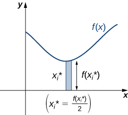
Figure $\PageIndex{8}$: A representative rectangle of the lamina.

Next, we need to find the total mass of the rectangle. Let $\rho$ represent the area density of the lamina (note that $\rho$ is a constant). Therefore, $\rho$ is expressed in mass per unit area. Thus, to find the total mass of the rectangle, we multiply the area of the rectangle by $\rho$. Then, the mass of the rectangle is given by $\rho f(x^∗_i) \Delta x$.

To get the approximate mass of the lamina, we add the masses of all the rectangles to get $$m \approx \sum_{i=1}^n \rho f(x^∗_i) \Delta x. \label{eq51}$$ Equation $\ref{eq51}$ is a Riemann sum. Taking the limit as $n \to \infty$ gives the exact mass of the lamina: $$\begin{array}{rcl} m & = & \displaystyle \lim_{n \to \infty }\sum_{i=1}^n \rho f(x^∗_i) \Delta x \\[12pt] & = & \rho \displaystyle \int^b_af(x)\,dx. \\ \end{array} \nonumber$$ Next, we calculate the moment of the lamina with respect to the $x$-axis. Returning to the representative rectangle, recall its center of mass is $\left(x^∗_i,\frac{f(x^∗_i)}{2}\right)$. Recall also that treating the rectangle as if it is a point mass located at the center of mass does not change the moment. Thus, the moment of the rectangle with respect to the $x$-axis is given by the mass of the rectangle, $\rho f(x^∗_i) \Delta x$, multiplied by the distance from the center of mass to the $x$-axis: $\frac{f(x^∗_i)}{2}$. Therefore, the moment with respect to the $x$-axis of the rectangle is $\rho \left( \frac{[f(x^∗_i)]^2}{2} \right) \Delta x.$ Adding the moments of the rectangles and taking the limit of the resulting Riemann sum, we see that the moment of the lamina with respect to the $x$-axis is $$\begin{array}{rcl} M_x & = & \displaystyle \lim_{n \to \infty }\sum_{i=1}^n \rho \dfrac{[f(x^∗_i)]^2}{2} \Delta x \\[12pt] & = & \rho \displaystyle \int ^b_a\dfrac{[f(x)]^2}{2}\,dx. \\ \end{array} \nonumber$$ We derive the moment with respect to the $y$-axis similarly, noting that the distance from the center of mass of the rectangle to the y-axis is $x^∗_i$. Then the moment of the lamina with respect to the $y$-axis is given by $$\begin{array}{rcl} M_y & = & \displaystyle \lim_{n \to \infty }\sum_{i=1}^n \rho x^∗_i f(x^∗_i) \Delta x \\[12pt] & = & \rho \displaystyle \int ^b_a x f(x) \, dx. \\ \end{array} \nonumber$$ We find the coordinates of the center of mass by dividing the moments by the total mass to give $\bar{x} = \frac{M_y}{m}$ and $\bar{y} = \frac{M_x}{m}$. If we look closely at the expressions for $M_x,M_y$, and $m$, we notice that the constant $\rho$ cancels out when $\bar{x}$ and $\bar{y}$ are calculated.

We summarize these findings in the following theorem.

Theorem: Center of Mass of a Thin Plate in the $xy$-Plane

Let $\mathbf{R}$ denote a region bounded above by the graph of a continuous function $f(x)$, below by the $x$-axis, and on the left and right by the lines $x=a$ and $x=b$, respectively. Let $\rho$ denote the area density of the associated lamina. Then we can make the following statements:

1. The mass of the lamina is $$m= \rho \int ^b_af(x) \, dx. \label{eq4a}$$
2. The moments $M_x$ and $M_y$ of the lamina with respect to the $x$- and $y$-axes, respectively, are $$M_x= \rho \int ^b_a\dfrac{[f(x)]^2}{2}dx\label{eq4b}$$ and $$M_y= \rho \int ^b_axf(x)dx.\label{eq4c}$$
3. The coordinates of the center of mass $(\bar{x},\bar{y})$ are $$\bar{x}=\dfrac{M_y}{m} \label{eq4d}$$ and $$\bar{y}=\dfrac{M_x}{m}. \label{eq4e}$$

In the next example, we use this theorem to find the center of mass of a lamina.

Example $\PageIndex{5}$: Finding the Center of Mass of a Lamina

Let $\mathbf{R}$ be the region bounded above by the graph of the function $f(x)=\sqrt{x}$ and below by the $x$-axis over the interval $[0,4]$. Find the centroid of the region.

Solution

The region is depicted in the following figure.

Figure $\PageIndex{9}$: Finding the center of mass of a lamina.

Since we are only asked for the region's centroid rather than the mass or moments of the associated lamina, we know the area density constant $\rho$ cancels out of the calculations eventually. Therefore, for the sake of convenience, let's assume $\rho =1$.

First, we need to calculate the total mass (Equation $\ref{eq4a}$): $$\begin{array}{rcl} m & = & \rho \displaystyle \int ^b_a f(x) \, dx \\[12pt] & = & \displaystyle \int ^4_0 \sqrt{x} \, dx \\[12pt] & = & \dfrac{2}{3}x^{3/2}\bigg|^4_0 \\[12pt] & = & \dfrac{2}{3}[8−0] \\[12pt] & = & \dfrac{16}{3}. \\ \end{array} \nonumber$$ Next, we compute the moments (Equation $\ref{eq4d}$): $$\begin{array}{rcl} M_x & = & \rho \displaystyle \int ^b_a\dfrac{[f(x)]^2}{2} \, dx \\[12pt] & = & \displaystyle \int ^4_0\dfrac{x}{2} \, dx \\[12pt] & = & \dfrac{1}{4}x^2\bigg|^4_0 \\[12pt] & = & 4 \\ \end{array} \nonumber$$ and (Equation $\ref{eq4c}$): $$\begin{array}{rcl} M_y & = & \rho \displaystyle \int ^b_a x f(x) \, dx \\[12pt] & = & \displaystyle \int ^4_0 x \sqrt{x} \, dx \\[12pt] & = & \displaystyle \int ^4_0 x^{3/2} \, dx \\[12pt] & = & \dfrac{2}{5} x^{5/2}\bigg|^4_0 \\[12pt] & = & \dfrac{2}{5}[32−0] \\[12pt] & = & \dfrac{64}{5}. \\ \end{array}\nonumber$$ Thus, we have (Equation $\ref{eq4d}$): $$\begin{array}{rcl} \bar{x} & = & \dfrac{M_y}{m} \\[12pt] & = & \dfrac{64/5}{16/3} \\[12pt] & = & \dfrac{64}{5} \cdot \dfrac{3}{16} \\[12pt] & = & \dfrac{12}{5} \\ \end{array} \nonumber$$ and (Equation $\ref{eq4e}$): $$\begin{array}{rcl} \bar{y} & = & \dfrac{M_x}{m} \\[12pt] & = & \dfrac{4}{16/3} \\[12pt] & = & 4 \cdot \dfrac{3}{16} \\[12pt] & = & \dfrac{3}{4}. \\ \end{array} \nonumber$$ The centroid of the region is $\left(\frac{12}{5}, \frac{3}{4}\right)$.

Checkpoint $\PageIndex{5}$

Let $\mathbf{R}$ be the region bounded above by the graph of the function $f(x)=x^2$ and below by the $x$-axis over the interval $[0,2].$ Find the centroid of the region.

Answer

The centroid of the region is $\left(\frac{3}{2}, \frac{6}{5}\right).$

We can also adapt this approach to find centroids of more complex regions. Suppose our region is bounded above by the graph of a continuous function $f(x)$, as before, but now, instead of having the lower bound for the region be the $x$-axis, suppose the region is bounded below by the graph of a second continuous function, $g(x)$, as shown in Figure $\PageIndex{10}$.

Figure $\PageIndex{10}$: A region between two functions.

Again, we partition the interval $[a,b]$ and construct rectangles. A representative rectangle is shown in Figure $\PageIndex{11}$.

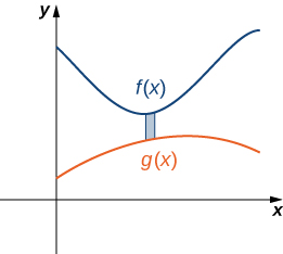
Figure $\PageIndex{11}$: A representative rectangle of the region between two functions.

Note that the centroid of this rectangle is $\left(x^∗_i, \frac{f(x^∗_i)+g(x^∗_i)}{2} \right)$. We won't go through all the details of the Riemann sum development, but let's look at some of the key steps. In the development of the formulas for the mass of the lamina and the moment with respect to the $y$-axis, the height of each rectangle is given by $y_T - y_B = f(x^∗_i)−g(x^∗_i)$, which leads to the expression $f(x)−g(x)$ in the integrands.

In the development of the formula for the moment with respect to the $x$-axis, the moment of each rectangle is found by multiplying the area density of the rectangle, $\rho [f(x^∗_i)−g(x^∗_i)] \Delta x$, by the distance of the centroid from the $x$-axis, $\frac{f(x^∗_i)+g(x^∗_i)}{2}$, which gives $\rho \frac{1}{2} \left[f(x^∗_i)]^2−[g(x^∗_i)]^2\right] \Delta x$. Summarizing these findings, we arrive at the following theorem.

Theorem: Center of Mass of a Lamina Bounded by Two Functions

Let $\mathbf{R}$ denote a region bounded above by the graph of a continuous function $f(x)$, below by the graph of the continuous function $g(x)$, and on the left and right by the lines $x=a$ and $x=b$, respectively. Let $\rho$ denote the area density of the associated lamina. Then we can make the following statements:

1. The mass of the lamina is $$m= \rho \int ^b_a[f(x)−g(x)] \, dx. \nonumber$$
2. The moments $M_x$ and $M_y$ of the lamina with respect to the $x$- and $y$-axes, respectively, are $$M_x= \rho \displaystyle \int ^b_a \frac{1}{2} \left([f(x)]^2−[g(x)]^2\right) \, dx \nonumber$$ and $$M_y= \rho \int ^b_a x [f(x)−g(x)] \, dx. \nonumber$$
3. The coordinates of the center of mass $(\bar{x},\bar{y})$ are $$\bar{x}=\dfrac{M_y}{m} \nonumber$$ and $$\bar{y}=\dfrac{M_x}{m}. \nonumber$$

We illustrate this theorem in the following example.

Example $\PageIndex{6}$: Finding the Centroid of a Region Bounded by Two Functions

Let $\mathbf{R}$ be the region bounded above by the graph of the function $f(x)=1−x^2$ and below by the graph of the function $g(x)=x−1.$ Find the centroid of the region.

Solution

The region is depicted in the following figure.

Figure $\PageIndex{12}$: Finding the centroid of a region between two curves.

The graphs of the functions intersect at $(−2,−3)$ and $(1,0)$, so we integrate from −2 to 1. Once again, for the sake of convenience, assume $\rho =1$.

First, we need to calculate the total mass: $$\begin{array}{rcl} m & = & \rho \displaystyle \int ^b_a[f(x)−g(x)] \, dx \\[12pt] & = & \displaystyle \int ^1_{−2}[1−x^2−(x−1)]\,dx \\[12pt] & = & \displaystyle \int ^1_{−2}(2−x^2−x) \, dx \\[12pt] & = & \left[2x−\dfrac{1}{3}x^3−\dfrac{1}{2}x^2\right]\bigg|^1_{−2} \\[12pt] & = & \left[2−\dfrac{1}{3}−\dfrac{1}{2}\right]−\left[−4+\dfrac{8}{3}−2\right] \\[12pt] & = & \dfrac{9}{2}. \\ \end{array} \nonumber$$ Next, we compute the moments: $$\begin{array}{rcl} M_x & = & \rho \displaystyle \int ^b_a\dfrac{1}{2}\left([f(x)]^2−[g(x)]^2\right) \, dx \\[12pt] & = & \dfrac{1}{2} \displaystyle \int ^1_{−2}((1−x^2)^2−(x−1)^2) \, dx \\[12pt] & = & \dfrac{1}{2} \displaystyle \int ^1_{−2}(x^4−3x^2+2x) \, dx \\[12pt] & = & \dfrac{1}{2} \left[\dfrac{x^5}{5}−x^3+x^2\right]\bigg|^1_{−2} \\[12pt] & = & −\dfrac{27}{10} \\ \end{array} \nonumber$$ and $$\begin{array}{rcl} M_y & = & \rho \displaystyle \int ^b_a x [f(x)−g(x)] \, dx \\[12pt] & = & \displaystyle \int ^1_{−2}x[(1−x^2)−(x−1)] \, dx \\[12pt] & = & \displaystyle \int ^1_{−2}x[2−x^2−x] \, dx \\[12pt] & = & \displaystyle \int ^1_{−2}(2x−x^4−x^2) \, dx \\[12pt] & = & \left[x^2−\dfrac{x^5}{5}−\dfrac{x^3}{3}\right]\bigg|^1_{−2} \\[12pt] & = & −\dfrac{9}{4}. \\ \end{array} \nonumber$$ Therefore, we have $$\begin{array}{rcl} \bar{x} & = & \dfrac{M_y}{m} \\[12pt] & = & −\dfrac{9}{4} \cdot \dfrac{2}{9} \\[12pt] & = & −\dfrac{1}{2} \\ \end{array} \nonumber$$ and $$\begin{array}{rcl} \bar{y} & = & \dfrac{M_x}{m} \\[12pt] & = & −\dfrac{27}{10} \cdot \dfrac{2}{9} \\[12pt] & = & −\dfrac{3}{5}. \\ \end{array} \nonumber$$ The centroid of the region is $\left(−\frac{1}{2},−\frac{3}{5}\right)$.

Checkpoint $\PageIndex{6}$

Let $\mathbf{R}$ be the region bounded above by the graph of the function $f(x)=6−x^2$ and below by the graph of the function $g(x)=3−2x.$ Find the centroid of the region.

Answer

The centroid of the region is $\left(1,\frac{13}{5}\right)$.

The Symmetry Principle

We stated the symmetry principle earlier when we were looking at the centroid of a rectangle. The symmetry principle can greatly help when finding centroids of symmetric regions. Consider the following example.

Example $\PageIndex{7}$: Finding the Centroid of a Symmetric Region

Let $\mathbf{R}$ be the region bounded above by the graph of the function $f(x)=4−x^2$ and below by the $x$-axis. Find the centroid of the region.

Solution

The region is depicted in the following figure

Figure $\PageIndex{13}$: We can use the symmetry principle to help find the centroid of a symmetric region.

The region is symmetric with respect to the $y$-axis. Therefore, the $x$-coordinate of the centroid is zero. We need only calculate $\bar{y}$. Once again, for the sake of convenience, assume $\rho =1$.

First, we calculate the total mass: $$\begin{array}{rcl} m & = & \rho \displaystyle \int ^b_a f(x) \, dx \\[12pt] & = & \displaystyle \int ^2_{−2}(4−x^2) \, dx \\[12pt] & = & \left[4x−\dfrac{x^3}{3}\right]\bigg|^2_{−2} \\[12pt] & = & \dfrac{32}{3}. \\ \end{array} \nonumber$$ Next, we calculate the moments. We only need $M_x$: $$\begin{array}{rcl} M_x & = & \rho \displaystyle \int ^b_a \dfrac{[f(x)]^2}{2} \, dx \\[12pt] & = & \dfrac{1}{2} \displaystyle \int ^2_{−2}\left[4−x^2\right]^2 \, dx \\[12pt] & = & \dfrac{1}{2} \displaystyle \int ^2_{−2}(16−8x^2+x^4) \, dx \\[12pt] & = & \dfrac{1}{2}\left[\dfrac{x^5}{5}−\dfrac{8x^3}{3}+16x\right]\bigg|^2_{−2} \\[12pt] & = & \dfrac{256}{15} \\ \end{array} \nonumber$$ Then we have $$\bar{y} = \dfrac{M_x}{m} = \dfrac{256}{15} \cdot \dfrac{3}{32} = \dfrac{8}{5}. \nonumber$$ The centroid of the region is $\left(0,\frac{8}{5}\right)$.

Checkpoint $\PageIndex{7}$

Let $\mathbf{R}$ be the region bounded above by the graph of the function $f(x)=1−x^2$ and below by $x$-axis. Find the centroid of the region.

Answer

The centroid of the region is $\left(0,\frac{2}{5}\right)$.

The Grand Canyon Skywalk

The Grand Canyon Skywalk opened on March 28, 2007. This engineering marvel is a horseshoe-shaped observation platform suspended 4000 ft above the Colorado River on the Grand Canyon's West Rim. Its crystal-clear glass floor allows stunning views of the canyon below (see the following figure).

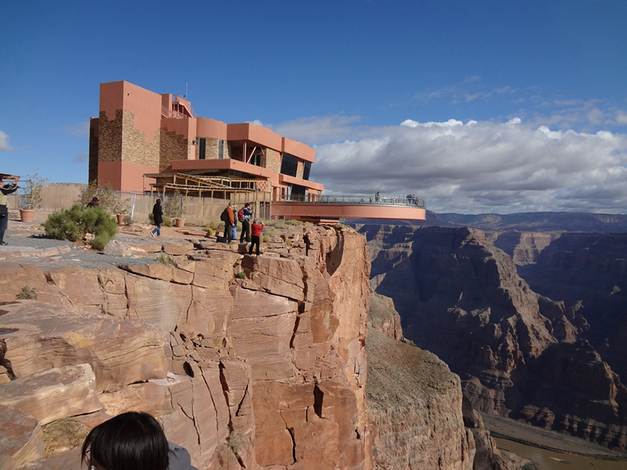
Figure $\PageIndex{14}$: The Grand Canyon Skywalk offers magnificent canyon views. (credit: 10da_ralta, Wikimedia Commons)

The Skywalk is a cantilever design, meaning that the observation platform extends over the canyon's rim with no visible means of support below it. Despite the lack of visible support posts or struts, cantilever structures are engineered to be very stable, and the Skywalk is no exception. The observation platform is attached firmly to support posts that extend 46 ft down into bedrock. The structure was built to withstand 100-mph winds and an 8.0-magnitude earthquake within 50 mi and is capable of supporting more than 70,000,000 lb.

One factor affecting the Skywalk's stability is the structure's center of gravity. We will calculate the center of gravity of the Skywalk and examine how the center of gravity changes when tourists walk out onto the observation platform.

The observation platform is U-shaped. The legs of the U are 10 ft wide and begin on land, under the visitors' center, 48 ft from the canyon's edge. The platform extends 70 ft over the edge of the canyon.

To calculate the center of mass of the structure, we treat it as a lamina and use a two-dimensional region in the $xy$-plane to represent the platform. We begin by dividing the area into three subregions so we can consider each subregion separately. The first region, denoted $\mathbf{R}_1$, consists of the curved part of the U. We model $\mathbf{R}_1$ as a semicircular annulus, with an inner radius of 25 ft and outer radius 35 ft, centered at the origin (Figure $\PageIndex{12}$).

Figure $\PageIndex{12}$: We model the Skywalk with three sub-regions.

The legs of the platform, extending 35 ft between $\mathbf{R}_1$ and the canyon wall, comprise the second sub-region, $\mathbf{R}_2$. Last, the ends of the legs, which extend 48 ft under the visitor center, comprise the third sub-region, $\mathbf{R}_3$. Assume the area density of the lamina is constant and assume the total weight of the platform is 1,200,000 lb (not including the weight of the visitor center; we will consider that later). Use $g=32\; \text{ft/sec}^2$.

1. Compute the area of each of the three sub-regions. Note that the areas of regions $\mathbf{R}_2$ and $\mathbf{R}_3$ should include the areas of the legs only, not the open space between them. Round answers to the nearest square foot.
2. Determine the mass associated with each of the three sub-regions.
3. Calculate the center of mass of each of the three sub-regions.
4. Now, treat each of the three sub-regions as a point mass located at the center of mass of the corresponding sub-region. Using this representation, calculate the center of mass of the entire platform.
5. Assume the visitor center weighs 2,200,000 lb, with a center of mass corresponding to the center of mass of $\mathbf{R}_3$. Treating the visitor center as a point mass, recalculate the system's center of mass. How does the center of mass change?
6. Although the Skywalk was built to limit the number of people on the observation platform to 120, the platform can support up to 800 people weighing 200 lb each. If all 800 people were allowed on the platform, and all of them went to the farthest end of the platform, how would the system's center of gravity be affected? (Include the visitor center in the calculations and represent the people by a point mass located at the farthest edge of the platform, 70 ft from the canyon wall.)

Theorem of Pappus

This section ends with a discussion of the Theorem of Pappus for volume, which allows us to find the volume of particular kinds of solids by using the centroid.²

Theorem of Pappus for Volume

Let $\mathbf{R}$ be a region in the plane and let $\mathcal{l}$ be a line in the plane that does not intersect $\mathbf{R}$. Then the volume of the solid of revolution formed by revolving $\mathbf{R}$ around $\mathcal{l}$ is equal to the area of $\mathbf{R}$ multiplied by the distance, $d$, traveled by the centroid of $\mathbf{R}$.

Proof

We can prove the case when the region is bounded above by the graph of a function $f(x)$ and below by the graph of a function $g(x)$ over an interval $[a,b]$, and for which the axis of revolution is the $y$-axis. In this case, the area of the region is $A= \displaystyle \int ^b_a[f(x)−g(x)]\,dx$. Since the axis of rotation is the $y$-axis, the distance traveled by the centroid of the region depends only on the $x$-coordinate of the centroid, $\bar{x}$, which is $$x=\dfrac{M_y}{m}, \nonumber$$ where $$m= \rho \int ^b_a[f(x)−g(x)] \, dx \nonumber$$ and $$M_y= \rho \int ^b_ax[f(x)−g(x)] \, dx. \nonumber$$ Then, $$d = 2 \pi \dfrac{ \rho \int ^b_ax[f(x)−g(x)] \, dx }{ \rho \int ^b_a[f(x)−g(x)] \, dx} \nonumber$$ and thus $$d \cdot A = 2 \pi \int ^b_ax[f(x)−g(x)] \, dx. \nonumber$$ However, using the Method of Cylindrical Shells, we have $$V = 2 \pi \int ^b_ax[f(x)−g(x)] \, dx. \nonumber$$ So, $$V=d \cdot A \nonumber$$ and the proof is complete.

Example $\PageIndex{8}$: Using the Theorem of Pappus for Volume

Let $\mathbf{R}$ be a circle of radius 2 centered at $(4,0).$ Use the Theorem of Pappus for Volume to find the volume of the torus generated by revolving $\mathbf{R}$ around the $y$-axis.

Solution

The region and torus are depicted in the following figure.

Figure $\PageIndex{15}$: Determining a torus's volume using the Pappus theorem. (a) A circular region $\mathbf{R}$ in the plane; (b) the torus generated by revolving $\mathbf{R}$ about the $y$-axis.

The region $\mathbf{R}$ is a circle of radius 2, so the area of $\mathbf{R}$ is $A=4 \pi \;\text{units}^2$. By the symmetry principle, the centroid of $\mathbf{R}$ is the circle's center. The centroid travels around the $y$-axis in a circular path of radius 4, so the centroid travels $d=8 \pi$ units. Then, the volume of the torus is $A \cdot d=32 \pi ^2 \, \text{units}^3$.

Checkpoint $\PageIndex{8}$

Let $\mathbf{R}$ be a circle of radius 1 centered at $(3,0).$ Use the Theorem of Pappus for Volume to find the volume of the torus generated by revolving $\mathbf{R}$ around the $y$-axis.

Answer

$6 \pi ^2 \, \text{units}^3$.

---

Footnotes

¹ A point mass refers to an idealized object that is considered to have mass but negligible size and shape.

² There is also a Theorem of Pappus for Surface Area, but it is much less useful than the theorem for volume.

---

Key Concepts

• Mathematically, the center of mass of a system is the point at which the system's total mass can be concentrated without changing the moment. Loosely speaking, the center of mass can be thought of as the balancing point of the system.
• For point masses distributed along a number line, the moment of the system with respect to the origin is $M=\sum^n_{i=1}m_ix_i.$ For point masses distributed in a plane, the moments of the system with respect to the $x$- and $y$-axes, respectively, are $M_x=\sum^n_{i=1}m_iy_i$ and $M_y=\sum^n_{i=}m_ix_i$, respectively.
• For a lamina bounded above by a function $f(x)$, the moments of the system with respect to the $x$- and $y$-axes, respectively, are $M_x= \rho \int ^b_a\dfrac{[f(x)]^2}{2}\,dx$ and $M_y= \rho \int ^b_axf(x)\,dx.$
• The $x$- and $y$-coordinates of the center of mass can be found by dividing the moments around the $y$-axis and around the $x$-axis, respectively, by the total mass. The symmetry principle says that if a region is symmetric with respect to a line, then the region's centroid lies on the line.
• The theorem of Pappus for volume says that if a region is revolved around an external axis, the volume of the resulting solid is equal to the area of the region multiplied by the distance traveled by the centroid of the region.

---

Key Equations

• Mass of a lamina

$m= \rho \int ^b_af(x)dx$

• Moments of a lamina

$M_x= \rho \int ^b_a\dfrac{[f(x)]^2}{2}\,dx\text{ and }M_y= \rho \int ^b_axf(x)\,dx$

• Center of mass of a lamina

$\bar{x}=\dfrac{M_y}{m}\text{ and }\bar{y}=\dfrac{M_x}{m}$

---

Glossary

center of mass

the point at which the total mass of the system could be concentrated without changing the moment

centroid

the centroid of a region is the geometric center of the region; laminas are often represented by regions in the plane; if the lamina has a constant density, the center of mass of the lamina depends only on the shape of the corresponding planar region; in this case, the center of mass of the lamina corresponds to the centroid of the representative region

lamina

a thin sheet of material; laminas are thin enough that, for mathematical purposes, they can be treated as if they are two-dimensional

moment

if n masses are arranged on a number line, the moment of the system with respect to the origin is given by $M=\sum^n_{i=1}m_ix_i$; if, instead, we consider a region in the plane, bounded above by a function $f(x)$ over an interval $[a,b]$, then the moments of the region with respect to the $x$- and $y$-axes are given by $M_x= \rho \int ^b_a\dfrac{[f(x)]^2}{2}\,dx$ and $M_y= \rho \int ^b_axf(x)\,dx$, respectively

symmetry principle

the symmetry principle states that if a region $R$ is symmetric about a line $I$, then the centroid of $R$ lies on $I$

theorem of Pappus for volume

this theorem states that the volume of a solid of revolution formed by revolving a region around an external axis is equal to the area of the region multiplied by the distance traveled by the centroid of the region