2.3: Integration by Parts

Note to the Instructor (click to expand) This is the standard Integration by Parts section with the inclusion of the integral of \( \sec^3(\theta)\) and power reduction formulas. It's fun and no-frills. The following is a list of learning objectives for this section. Learning Objectives (click to expand) Recognize when to use Integration by Parts. Use the Integration by Parts formula to solve integration problems. Use the Integration by Parts formula for definite integrals.

Hawk A.I. Section-Specific Tutor To access the Hawk A.I. Tutor, you will need to be logged into your campus Gmail account.

By now, we have a fairly thorough procedure for evaluating many basic integrals. However, although we can integrate \( \int x \sin (x^2)\,dx\) by using the substitution, \(u=x^2\), something as simple looking as \( \int x\sin x\,\,dx\) defies us. Many students want to know whether there is a Product Rule for integration. There is not, but a technique based on the Product Rule for differentiation allows us to exchange one integral for another. We call this technique Integration by Parts.

The Integration by Parts Formula

If, \(h(x)=f(x)g(x)\), then by using the Product Rule, we obtain\[h^{\prime}(x)=f^{\prime}(x)g(x)+g^{\prime}(x)f(x). \label{eq1} \]Although at first it may seem counterproductive, let's now integrate both sides of Equation \ref{eq1}:\[ \int h^{\prime}(x)\,\,dx= \int (g(x)f^{\prime}(x)+f(x)g^{\prime}(x))\,\, dx. \nonumber \]This gives us\[ h(x)=f(x)g(x)= \int g(x)f^{\prime}(x)\,dx+ \int f(x)g^{\prime}(x)\,\,dx. \nonumber \]Now we solve for \( \int f(x)g^{\prime}(x)\,\,dx\):\[ \int f(x)g^{\prime}(x)\,dx=f(x)g(x)− \int g(x)f^{\prime}(x)\,\,dx. \nonumber \]By making the substitutions \(u=f(x)\) and \(v=g(x)\), which in turn make \(du=f^{\prime}(x)\,dx\) and \(dv=g^{\prime}(x)\,dx\), we have the more compact form\[ \int u\,dv=uv− \int v\,du. \nonumber \]

Theorem: Integration by Parts

Let \(u=f(x)\) and \(v=g(x)\) be functions with continuous derivatives. Then, the Integration by Parts formula (also known as IbP) for the integral involving these two functions is:\[ \int u\,dv=uv− \int v\, du. \label{IBP} \]

The advantage of using the Integration by Parts formula is that we can exchange one integral for another, possibly more accessible integral. The following example illustrates its use.

Example \(\PageIndex{1}\): Using Integration by Parts

Use Integration by Parts with \(u=x\) and \(dv=\sin x\,\,dx\) to evaluate\[ \int x\sin x\,\,dx. \nonumber \]

Solution

By choosing \(u=x\), we have \(du=1\,\,dx\). Since \(dv=\sin x\,\,dx\), we get\[v= \int \sin x\,\,dx=−\cos x. \nonumber \]It is handy to keep track of these values in a table, as follows:

\( u = x \)	\( dv = \sin x \, dx \)
\( du = 1\, dx \)	\( v = \int \sin x \, dx = - \cos x \)

Applying the Integration by Parts formula (Equation \ref{IBP}) results in\[ \begin{array}{rclcl}
\displaystyle \int x\sin x\,\,dx & = & (x)(−\cos x) − \displaystyle \int (−\cos x)(1\,\,dx) & \quad & \left( \text{substitution} \right) \\[12pt]
& = & −x\cos x+ \displaystyle \int \cos x\,\,dx & \quad & \left(\text{simplifying} \right) \\
\end{array} \nonumber \]Then use\[ \int \cos x\,\,dx =\sin x+C \nonumber \]to obtain\[ \int x\sin x\,\,dx =−x\cos x+\sin x+C. \nonumber \]

Analysis

At this point, a few items need clarification. First, what would have happened if we had chosen \(u=\sin x\) and \(dv=x,\ dx\)? If we had done so, then we would have \(du=\cos x \, dx\) and \(v=\frac{1}{2}x^2\). Thus, after applying Integration by Parts (Equation \ref{IBP}), we have\[ \int ​x\sin x\,\,dx=\dfrac{1}{2}x^2\sin x− \int \dfrac{1}{2}x^2\cos x\,\,dx. \nonumber \]Unfortunately, we are in no better position than before with the new integral. It is important to remember that when we apply Integration by Parts, we may need to try several choices for \(u\) and \(dv\) before finding a choice that works.

Second, you may wonder why, when we find \(v= \int ​\sin x\,\,dx=−\cos x\), we do not use \(v=−\cos x+K\). To see that it makes no difference, we can rework the problem using \(v=−\cos x+K\):\[ \begin{array}{rcl}
\displaystyle \int x\sin x\,\,dx & = & (x)(−\cos x+K)− \int (−\cos x+K)(1\,\,dx) \\[12pt]
& = & −x\cos x+Kx+ \displaystyle \int \cos x\,\,dx− \int K\,\,dx \\[12pt]
& = & −x\cos x+Kx+\sin x−Kx+C \\[12pt]
& = & −x\cos x+\sin x+C. \\
\end{array} \nonumber \]As you can see, it makes no difference in the final solution.

Last, we can check to make sure that our antiderivative is correct by differentiating \(−x\cos x+\sin x+C\):\[ \begin{array}{rcl}
\dfrac{d}{\,dx}(−x\cos x+\sin x+C) & = & \cancel{(−1)\cos x} + (−x)(−\sin x) + \cancel{\cos x} \\[12pt]
& = & x\sin x \\
\end{array} \nonumber \]Therefore, the antiderivative checks out.

Checkpoint \(\PageIndex{1}\)

Evaluate \( \int ​xe^{2x}\,dx\) using the Integration by Parts formula (Equation \ref{IBP}) with \(u=x\) and \(dv=e^{2x}\,\,dx\).

Answer

\[ \int ​xe^{2x}\,\,dx=\dfrac{1}{2}xe^{2x}−\dfrac{1}{4}e^{2x}+C \nonumber \]

Choosing \( u \) and \( dv \)

The natural question to ask at this point is: How do we know what to choose for \(u\) and \(dv\)?

Most authors will immediately give you a trick to picking the "right" choice for \( u \); however, the trick they give is not flawless. It often fails. Therefore, it is best to develop an approach to Integration by Parts from the other direction - by asking, "What is a good choice for \( dv \)?

Our choice for \( dv \) will immediately inform us as to what \( u \) needs to be. Since we are going to have to integrate \( dv \), you want to choose it to be something you actually can integrate. This is so important that it bears repeating:

Integration by Parts boils down to selecting a factor, preferably the most complex, of the integrand that you can integrate either by direct integration or by the Substitution Method.

That's it! The rest of this subsection discusses why we make certain choices for \( dv \) and \( u \). Still, in the end, it's all about asking yourself, "What's the most complex factor of this integrand I can integrate?"

Now, think of all of the "traditional" functions you have encountered up to this point in mathematics, and ask yourself which ones you can easily integrate.

Basic Function Type	Easily Integrable?
Algebraic (e.g., \( x^3 \), \( \sqrt{x} \), and \( \frac{1}{x} \))	Yes
Exponential (e.g., \( e^x \) and \( 2^x \) )	Yes
Logarithmic (e.g., \( \ln(x) \) and \( \log_3(x) \))	No
Trigonometric (e.g., \( \sin(x) \) and \( \sec^2(x) \), but not \( \sec(x) \))	Yes (in some cases)
Inverse Trigonometric (e.g., \( \tan^{-1}(x) \) and \( \csc^{-1}(x) \))	No

Since we do not have integration formulas that allow us to integrate simple Logarithmic functions and Inverse trigonometric functions,¹ it makes sense that they should not be chosen for \(dv\). On the other hand, Exponential and Trigonometric functions are, in general, easy to integrate and make good choices for \(dv\). Finally, we can always integrate basic Algebraic functions. However, their antiderivatives require slightly more work than the straightforward antiderivatives of the exponential and trigonometric functions. Therefore, if given the option, we would rather integrate exponential or trigonometric functions than algebraic functions.

Given that discussion, we have the following tactic.

Tactic for Choosing \( dv \)

Given an integral where you wish to use Integration by Parts, the order of preference for choosing \( dv \) is as follows:

1. Exponential functions
2. Trigonometric functions
3. Algebraic functions
4. Inverse trigonometric functions
5. Logarithmic functions

As was mentioned previously, most authors approach this conversation by stating what your choice of \( u \) should be rather than \( dv \). To accommodate students with instructors who take this same approach, we could reverse the direction of our tactic for choosing \( dv \) and, instead, create the commonly-taught tactic for choosing \( u \). If logarithms are the worst choice for \( dv \), then they will be our first choice for \( u \), and so on. This gives us the following tactic for choosing \( u \).

Tactic for Choosing \( u \)

Given an integral where you wish to use Integration by Parts, the order of preference for choosing \( u \) is as follows:

1. Logarithmic functions
2. Inverse trigonometric functions
3. Algebraic functions
4. Trigonometric functions
5. Exponential functions

This last tactic gives a common mnemonic, LIATE, to take some of the guesswork out of our choices for \( u \). The type of function in the integral that appears first in the list should be our first choice of \(u\).² When we have chosen \(u\), \(dv\) is selected to be the remaining part of the integrand.

Caution: My Approach

I stick with finding \( dv \) first instead of finding \( u \) so that you get a more natural and understandable approach to Integration by Parts. All of the examples will reflect this.

Thus, if an integral contains the product of a logarithmic function and an algebraic function, we would choose \( dv \) to be the algebraic function (because we don't know how to integrate a logarithm as of yet). Therefore, we would choose \( u \) to be the logarithmic function. Following the typical textbook tactic, our choice for \( u \) is correct because L comes before A in LIATE.

The integral in Example \(\PageIndex{1}\) has a trigonometric function, \(\sin x\), and an algebraic function, \(x\). Both of these are easily integrable, but we would rather integrate \( \sin x \) over \( x \) because antiderivatives of trigonometric functions are simple (as opposed to algebraic functions, which require raising powers and dividing by new powers). Thus, we would choose \( dv = \sin x \, dx \) and \( u = x \). Again, this coincides with our decision to use the common textbook tactic because A comes before T in LIATE.

There is a second, more important reason as to why we are selecting to differentiate the algebraic function and integrate the trigonometric function in Example \( \PageIndex{1} \). When we tried to go the opposite direction (choosing to integrate the algebraic function and differentiate the trigonometric function), we arrived at an integral that got worse as we ended with an algebraic function of higher power and we still had a trigonometric function. A hidden goal when dealing with products of polynomials and other functions is to remove the polynomial. This can only be done if we take derivatives of the polynomial. While this might seem confusing right now, things will get more apparent as you use Integration by Parts.

Finally, here is the rule of thumb I tell my students:

Rule of Thumb: Choosing \( dv \) and \( u \)

When using Integration by Parts:

• Choose \( dv \) to be the largest factor of the integrand that you can integrate, either directly or by using the Substitution Method - \( u \) will be the rest of the integrand. You will often need to rewrite the integrand to see this largest factor and, remember, \( \int f(x) \, dx = \int f(x) \cdot 1 \, dx \). This is especially useful if you cannot integrate any obvious factor within the integrand.
• If you can integrate all factors within the integrand, then switch gears and instead choose \( u \) to be the factor whose derivative (or eventual, higher-order derivative) changes forms or becomes a constant.
• If you have to use Integration by Parts more than once while evaluating an integral, be sure to stay with the same "function type" choice for all Integrations by Parts.

The best way to understand this Rule of Thumb is through examples.

Example \(\PageIndex{2}\): Using Integration by Parts

Evaluate \[ \int \dfrac{\ln x}{x^3}\,\,dx. \nonumber \]

Solution

\( \boxed{\times} \) Direct Integration: Since the integrand is not the derivative of an established, well-known function, we cannot directly integrate.

\( \boxed{\times} \) Simple \( u \)-Substitution: I leave it for the reader to try as they might to find a proper \( u \)-substitution - none will work.

\( \boxed{\times} \) Radical Substitution: Since a simple \( u \)-substitution will not work, a radical substitution is out of the question.

\( \boxed{\times} \) Trigonometric Substitution: As written, there isn't any obvious trigonometric substitution.

\( \boxed{?} \) By Parts: Since the integrand is the product of two different function types, it is a good candidate for Integration by Parts.³

It is helpful, at times, to begin by rewriting the integral:\[ \int \dfrac{\ln x}{x^3}\,\,dx= \int ​x^{−3}\ln x\,\, dx. \nonumber \]Consider the factors of the integrand - \( x^{-3} \) and \( \ln(x) \). Which one can we easily integrate? The obvious answer here is \( x^{-3} \). Hence, we choose \( dv = x^{-3} \, dx \) (don't forget the \( dx \)) and we let \( u \) be the rest of the integrand. That is, \( u = \ln(x) \).

For the LIATE Folks

We choose \(u=\ln x\) and \( dv = x^{-3} \, dx \), since L comes before A in LIATE.

Next, since \(u=\ln x,\) we have \(du=\frac{1}{x}\,dx\). Also, \(v= \int ​x^{−3}\,dx=−\frac{1}{2}x^{−2}\). Summarizing,

\( u = \ln(x) \)	\( dv = x^{-3} \, dx \)
\( du = \dfrac{1}{x} \, dx \)	\( v = -\dfrac{1}{2} x^{-2} \)

Substituting into the Integration by Parts formula (Equation \ref{IBP}) gives\[ \begin{array}{rcl}
\displaystyle \int \dfrac{\ln x}{x^3}\,dx & = & \int ​x^{−3}\ln x\,dx \\[12pt]
& = & \left(\ln x\right)\left(−\dfrac{1}{2}x^{−2}\right)− \displaystyle \int ​\left(−\dfrac{1}{2}x^{−2}\right)\left(\dfrac{1}{x}\,dx\right) \\[12pt]
& = & −\dfrac{1}{2}x^{−2}\ln x+ \displaystyle \int \dfrac{1}{2}x^{−3}\,dx \\[12pt]
& = & −\dfrac{1}{2}x^{−2}\ln x−\dfrac{1}{4}x^{−2}+C \\[12pt]
& = & −\dfrac{1}{2x^2}\ln x−\dfrac{1}{4x^2}+C \\
& & \\
\end{array} \nonumber \]

Checkpoint \(\PageIndex{2}\)

Evaluate \[ \int ​x \ln x \, dx. \nonumber \]

Answer

\[ \int ​x\ln x \,\,dx=\dfrac{1}{2}x^2\ln x−\dfrac{1}{4}x^2+C \nonumber \]

More Complex Uses of Integration by Parts

In some cases, as in the next two examples, it may be necessary to apply Integration by Parts more than once.

Example \(\PageIndex{3}\): Applying Integration by Parts More Than Once

Evaluate\[ \int ​x^2e^{3x}\,dx. \nonumber \]

Solution

\( \boxed{\times} \) Direct Integration: Since the integrand is not the derivative of an established, well-known function, we cannot directly integrate.

\( \boxed{\times} \) Simple \( u \)-Substitution: I leave it for the reader to try as they might to find a proper \( u \)-substitution - none will work.

\( \boxed{\times} \) Radical Substitution: Since a simple \( u \)-substitution will not work, a radical substitution is out of the question.

\( \boxed{\times} \) Trigonometric Substitution: As written, there isn't any obvious trigonometric substitution.

\( \boxed{?} \) By Parts: Since the integrand is the product of two different function types, it is a good candidate for Integration by Parts.

Since we can easily integrate both \( x^2 \) and \( e^{3x} \), we switch gears and ask ourselves which one has a derivative (or eventual, higher-order derivative) that will change forms. Thus, we choose \( u = x^2 \) because a couple of derivatives will result in the function completely devolving into a constant function. Therefore, \( dv = e^{3x} \, dx \).

\( u = x^2 \)	\( dv = e^{3x} \, dx \)
\( du = 2x \, dx \)	\( v = \dfrac{1}{3} e^{3x} \)

For the LIATE Folks

Choose \(u=x^2\) and \(dv=e^{3x}\,dx\) because A comes before E in LIATE.

Substituting into Equation \ref{IBP} produces\[ \int x^2e^{3x}\,dx = \dfrac{1}{3}x^2e^{3x} − \int \dfrac{2}{3}xe^{3x}\,dx = \dfrac{1}{3}x^2e^{3x} − \dfrac{2}{3} \int xe^{3x}\,dx. \label{3A.2} \]We still cannot integrate \( \displaystyle \int xe^{3x}\, dx\) directly, but the integral now has a lower power on \(x\). We can evaluate this new integral by using Integration by Parts again. Since we have already started the Integration by Parts process on this integral, we stick with the same "function type" choices for \( u \) and \( dv \). We chose \( u \) to be the algebraic function on our first Integration by Parts, so our choice of \( u \) on this new Integration by Parts must also be an algebraic function.

For the LIATE Folks

Choose \(u=x\) and \(dv=e^{3x}\,dx\) because A comes before E in LIATE.

\( u = x \)	\( dv = e^{3x} \, dx \)
\( du = dx \)	\( v = \dfrac{1}{3} e^{3x} \)

Substituting back into Equation \ref{3A.2} yields\[ \int ​x^2e^{3x}\,dx = \dfrac{1}{3}x^2e^{3x}− \dfrac{2}{3} \left(\dfrac{1}{3}xe^{3x}− \int \dfrac{1}{3}e^{3x}\,dx\right). \nonumber \]After evaluating the last integral and simplifying, we obtain\[ \int x^2e^{3x}\,dx=\dfrac{1}{3}x^2e^{3x}−\dfrac{2}{9}xe^{3x}+\dfrac{2}{27}e^{3x}+C. \nonumber \]

Example \( \PageIndex{3} \) showcases a vital difference between LIATE and having a more natural understanding of Integration by Parts using the Rule of Thumb. When using LIATE, we chose \( u = x^2 \) by rote memorization without understanding the consequences of the choice. The Rule of Thumb, on the other hand, delivered an extra bit of "hidden" knowledge - since we chose \( u = x^2 \) because it changes form after two derivatives, we could have immediately recognized that this integral would require two integrations (in this case, two applications of Integration by Parts).

Example \(\PageIndex{4}\): Applying Integration by Parts When LIATE Does not Quite Work

Evaluate\[ \int ​t^3e^{t^2}\, dt. \nonumber \]

Solution

\( \boxed{\times} \) Direct Integration: Since the integrand is not the derivative of an established, well-known function, we cannot directly integrate.

\( \boxed{?} \) Simple \( u \)-Substitution: Letting \( u = t^2 \) might work.

\( \boxed{\times} \) Radical Substitution: There is not a radical in the integrand.

\( \boxed{\times} \) Trigonometric Substitution: As written, there isn't any obvious trigonometric substitution.

\( \boxed{?} \) By Parts: Since the integrand is the product of two different function types, it is a good candidate for Integration by Parts.

This is an excellent example of having many approaches to a problem that are all correct - welcome to the wonderful world of real integration!

Approach #1 (Ineffective): Using LIATE

For the LIATE-lovers out there, this one's for you. If we use a strict interpretation of the mnemonic LIATE to make our choice of \(u\), we end up with \(u=t^3\) and \(dv=e^{t^2} \, dt\).

\( u = t^3 \)	\( dv = e^{t^2} \, dt \)
\( du = 3t^2 \, dt \)	\( v = \ldots \left( \text{we're stuck} \right) \)

Unfortunately, we cannot continue with this approach because we cannot integrate \( e^{t^2} \).

Approach #2: Starting with a Substitution

Using the Substitution Method, we could let \( w = t^2 \) so that \( dw = 2 t \, dt \). This means \( \frac{1}{2} dw = t \, dt \). Hence,\[ \begin{array}{rclccl}
\displaystyle \int t^3 e^{t^2} \, dt & = & \displaystyle \int t^2 e^{t^2} t \, dt & & \\[12pt]
& = & \dfrac{1}{2} \displaystyle \int w e^w \, dw & \quad & \left( \text{substituting }w = t^2 \implies \dfrac{1}{2} dw = t \, dt \right) \\
\end{array} \nonumber \]We can integrate both \( w \) and \( e^w \), so we focus on choosing \( u \) to be the factor whose derivative (or eventual derivative) changes form. This is \( w \). Thus, we choose \( u = w \) and \( dv = e^w \, dw \).

\( u = w \)	\( dv = e^w \, dw \)
\( du = dw \)	\( v = e^w \)

Using Integration by Parts, we get\[ \begin{array}{rclcl}
\displaystyle \int t^3 e^{t^2} \, dt & = & \displaystyle \int t^2 e^{t^2} t \, dt & & \\[12pt]
& = & \dfrac{1}{2} \displaystyle \int w e^w \, dw & \quad & \left( \text{substituting }w = t^2 \implies \dfrac{1}{2} dw = t \, dt \right) \\[12pt]
& = & \dfrac{1}{2} \left( w e^w - \displaystyle \int e^w \, dw \right) & \quad & \left( \text{IbP} \right) \\[12pt]
& = & \dfrac{1}{2} \left( w e^w - e^w + C_1\right) & & \\[12pt]
& = & \dfrac{1}{2} \left( t^2 e^{t^2} - e^{t^2} + C_1 \right) & \quad & \left( \text{resubstituting }w = t^2 \right) \\[12pt]
& = & \dfrac{1}{2} t^2 e^{t^2} - \dfrac{1}{2} e^{t^2} + C & \quad & \left( \dfrac{1}{2} C_1 \text{ is a constant, so we call it }C \right) \\
\end{array} \nonumber \]

Approach #3 (Most Efficient): Starting with IBP by Choosing \( dv \) to be the Largest Integrable Factor

If we rewrite the given integral as\[ \int t^2 \left( t e^{t^2} \right) \, dt, \nonumber \]we can see that both \( t^2 \) and \( t e^{t^2} \) are integrable. Therefore, we choose \( dv \) to be the "larger" (read as "more complex") of these two factors. Hence, we choose \( dv = t e^{t^2} \, dt \) and \( u = t^2 \).⁴

\( u = t^2 \)	\( dv = t e^{t^2} \, dt \)
\( du = 2 t \, dt \)	\( v = \dfrac{1}{2} e^{t^2} \) (Substitution Method)

Therefore, we get\[ \begin{array}{rclcl}
\displaystyle \int t^3e^{t^2} \, dt & = & \displaystyle \int t^2 \left(t e^{t^2}\right) \, dt & & \\[12pt]
& = & \dfrac{1}{2} t^2 e^{t^2} - \displaystyle \int t e^{t^2} \, dt. & \quad & \left( \text{IbP} \right) \\[12pt]
& = & \dfrac{1}{2} t^2 e^{t^2} - \dfrac{1}{2} e^{t^2} + C & & \\
\end{array} \nonumber \]

There are a couple of things I want to mention about Example \( \PageIndex{4} \). First, notice that LIATE failed us here, but a natural understanding of our goal - to find the largest factor of the integrand that we can integrate - still led us to a solution. This is why I do not teach LIATE in my classes (again, I only include it here because you will hear of it from students in other classes, and those students might have the illusion that it always works).

The second thing to mention is that Approach #3 in this example demonstrates the level of comfort with integration for which you want to strive. There is nothing wrong with Approach #2, but you definitely want to build the skill set to perform complex integrations like this. However, The only way you will build that skill is through lots of practice!

Caution: Practice Makes Better

Integration by Parts (and most other integration techniques) is almost a completely heuristic method. That is, you will only learn how to identify when to use a technique properly and what pitfalls to avoid by practicing.

Example \(\PageIndex{5}\): Self-Relating Integration by Parts

Evaluate\[ \int ​\sin (\ln x)\,dx. \nonumber \]

Solution

\( \boxed{\times} \) Direct Integration: Since the integrand is not the derivative of an established, well-known function, we cannot directly integrate.

\( \boxed{\times} \) Simple \( u \)-Substitution: I leave it for the reader to try as they might to find a proper \( u \)-substitution - none will work.

\( \boxed{\times} \) Radical Substitution: Since a simple \( u \)-substitution will not work, a radical substitution is out of the question.

\( \boxed{\times} \) Trigonometric Substitution: As written, there isn't any obvious trigonometric substitution.

\( \boxed{?} \) By Parts: Since the integrand is not the product of two different function types, it doesn't seem to be a good candidate for Integration by Parts.⁵

Again, LIATE fails us here, but the Rule of Thumb is still helpful. We begin by rewriting the integral as\[ \int ​\sin (\ln x) \cdot 1 \, dx. \nonumber \]We can integrate \( 1 \), but not \( \sin(\ln(x)) \), so we let \( dv = 1 \, dx \).

\( u = \sin(\ln(x)) \)	\( dv = 1 \, dx \)
\( du = \dfrac{\cos(\ln(x))}{x} \, dx \)	\( v = x \)

Therefore, we have\[ \int ​\sin \left(\ln (x)\right) \,dx = x \sin (\ln (x)) − \int \cos (\ln (x))\,dx. \nonumber \]Unfortunately, this process leaves us with a new integral that is very similar to the original. However, let's see what happens when we apply Integration by Parts again.

Since we chose \( u \) to be the composition of the trigonometric function and the logarithmic function on our first pass of the Integration by Parts method, we choose the same style of function for \( u \) on our second pass.

\( u = \cos(\ln(x)) \)	\( dv = 1 \, dx \)
\( du = -\dfrac{\sin(\ln(x))}{x} \, dx \)	\( v = x \)

Substituting, we have\[ \int ​\sin (\ln (x))\,dx = x \sin (\ln x)−\left(x \cos (\ln (x)) - \int -​\sin (\ln (x))\,dx\right). \nonumber \]After simplifying, we obtain\[ \int ​\sin (\ln (x))\,dx=x\sin (\ln (x))−x \cos (\ln (x))− \int ​\sin (\ln (x))\,dx. \nonumber \]The last integral is now the same as the original. It may seem that we have gone in circles, but now we can evaluate the integral. To see how to do this more clearly, substitute \(I= \int ​\sin (\ln (x))\,dx.\) Thus, the equation becomes\[I=x \sin (\ln (x))−x \cos (\ln (x))−I. \nonumber \]First, add \(I\) to both sides of the equation to obtain\[2I=x \sin (\ln (x))−x \cos (\ln (x)). \nonumber \]Next, divide by 2:\[I=\dfrac{1}{2}x \sin (\ln (x))−\dfrac{1}{2}x \cos (\ln (x)). \nonumber \]Substituting \(I= \int ​\sin (\ln (x))\,dx\) again, we have\[ \int \sin (\ln (x)) \,dx=\dfrac{1}{2}x \sin (\ln (x))−\dfrac{1}{2}x \cos (\ln (x)). \nonumber \]From this we see that \(\frac{1}{2}x \sin (\ln (x))−\frac{1}{2}x \cos (\ln (x))\) is an antiderivative of \(\sin (\ln (x))\). For the most general antiderivative, add \(C\):\[ \int \sin (\ln (x)) \,dx=\dfrac{1}{2}x \sin (\ln (x))−\dfrac{1}{2}x \cos (\ln (x))+C. \nonumber \]

Analysis

If this method feels a little strange at first, we can check the answer by differentiation:\[\begin{array}{rcl}
\dfrac{d}{\,dx}\left(\dfrac{1}{2}x \sin (\ln x)−\dfrac{1}{2}x\cos (\ln x)\right) & = & \dfrac{1}{2}(\sin (\ln x))+\cos (\ln x) \cdot \dfrac{1}{x} \cdot \dfrac{1}{2}x−\left(\dfrac{1}{2}\cos (\ln x)−\sin (\ln x) \cdot \dfrac{1}{x} \cdot \dfrac{1}{2}x\right) \\[12pt]
& = & \sin (\ln x). \\
\end{array} \nonumber \]

Example \( \PageIndex{ 5 } \) is an integral I call a "Self-Relating Integration by Parts." This is because, when we use Integration by Parts, we obtain the original integral as part of our evaluated integral. This style of integration comes up frequently enough that you should practice it until it is comfortable.

Checkpoint \(\PageIndex{5}\)

Evaluate\[ \int x^2\sin x\,dx. \nonumber \]

Answer

\[ \int x^2\sin x\,dx=−x^2\cos x+2x\sin x+2\cos x+C \nonumber \]

In Section 2.1, we introduced the following Problem-Solving Strategy for dealing with integrals involving products of powers of the tangent and secant functions. In this case, we complete the strategy by filling out the fourth tactic - one that requires Integration by Parts.

Problem-Solving Strategy: Integrating \(\displaystyle \int \tan^k(x)\sec^j(x)\,dx\)

To integrate \(\displaystyle \int \tan^k(x)\sec^j(x)\,dx,\) use the following strategies:

1. If \(j\) is even and \(j \geq 2,\) rewrite \(\sec^j(x)=\sec^{j−2}(x)\sec^2(x)\) and use \(\sec^2(x)=\tan^2(x)+1\) to rewrite \(\sec^{j−2}(x)\) in terms of \(\tan(x)\). Let \(u=\tan(x)\) and \(du=\sec^2(x)\,dx\).
2. If \(k\) is odd and \(j \geq 1\), rewrite \(\tan^k(x)\sec^j(x)=\tan^{k−1}(x)\sec^{j−1}(x)\sec(x)\tan(x)\) and use \(\tan^2(x)=\sec^2(x)−1\) to rewrite \(\tan^{k−1}(x)\) in terms of \(\sec(x)\). Let \(u=\sec(x)\) and \(du=\sec(x)\tan(x)\, dx.\) (Note: If \(j\) is even and \(k\) is odd, then either strategy 1 or strategy 2 may be used.)
3. If \(k\) is odd where \(k \geq 3\) and \(j=0\), rewrite \(\tan^k(x)=\tan^{k−2}(x)\tan^2(x)=\tan^{k−2}(x)(\sec^2(x)−1)=\tan^{k−2}(x)\sec^2(x)−\tan^{k−2}(x)\). It may be necessary to repeat this process on the \(\tan^{k−2}(x)\) term.
4. If \(k\) is even and \(j\) is odd, then use \(\tan^2(x)=\sec^2(x)−1\) to express \(\tan^k(x)\) in terms of \(\sec(x)\). Use Integration by Parts to integrate odd powers of \(\sec(x).\)

Example \(\PageIndex{6}\): Integrating \( \sec^3(x)\)

Evaluate \(\displaystyle \int \sec^3(x)\,dx\).

Solution

\( \boxed{\times} \) Direct Integration: Since the integrand is not the derivative of an established, well-known function, we cannot directly integrate.

\( \boxed{\times} \) Simple \( u \)-Substitution: Any choice of substitution will lead nowhere. For example, letting \( u = \tan(x) \) will definitely "steal" two powers off the secant (via \( du = \sec^2(x) \, dx \)); however, the secant would be left with an odd power - we don't want that. Letting \( u = \sec(x) \) would steal a power off tangent (via \( du = \sec(x) \tan(x) \, dx \)), leaving \( \left( \tan(x) \right)^{-1} \); however, we would need that power on tangent to be even, and that's not going to happen. I leave it for the reader to try as they might to find a proper \( u \)-substitution - none will work.

\( \boxed{\times} \) Radical Substitution: The integrand doesn't involve a radical.

\( \boxed{\times} \) Trigonometric Substitution: As written, there isn't any obvious trigonometric substitution.

\( \boxed{?} \) By Parts: Since all other techniques have failed, we might be able to use Integration by Parts; however, as written, we have no clue where to start.

This integral is dangerously popular in some texts!

Since we are stuck from the get-go, let's use the Mathematical Mantra and see if there is anything from Trigonometry that might help. We would like to rewrite the integrand as the product of two functions (which is not technically always needed for Integration by Parts, but it is helpful here):\[ \int \sec^3(x) \, dx = \int \sec(x) \sec^2(x) \, dx. \nonumber \]We definitely can integrate \( sec^2(x) \), so we choose \( dv = \sec^2(x) \, dx \) and \( u = \sec(x) \).

\( u = \sec(x) \)	\( dv = \sec^2(x) \, dx \)
\( du = \sec(x) \tan(x) \, dx \)	\( v = \tan(x) \)

Thus,\[\begin{array}{rcl}
\displaystyle \int \sec^3(x)\,dx & = & \sec(x)\tan(x) − \displaystyle \int \tan(x)\sec(x)\tan(x)\,dx \\[6pt]
& = & \sec(x)\tan(x) − \displaystyle \int \tan^2(x)\sec(x)\,dx \\[6pt]
& = & \sec(x)\tan(x) − \displaystyle \int (\sec^2(x)−1)\sec(x)\,dx \\[6pt]
& = & \sec(x)\tan(x) + \displaystyle \int \sec(x)\,dx − \displaystyle \int \sec^3(x)\,dx \\[6pt]
& = & \sec(x)\tan(x) + \ln|\sec(x)+\tan(x)| − \displaystyle \int \sec^3(x)\,dx. \\[6pt]
\end{array} \nonumber \]We now have\[ \int \sec^3(x)\,dx=\sec(x)\tan(x)+\ln|\sec(x)+\tan(x)|− \int \sec^3(x)\,dx.\nonumber \]Since the integral \(\displaystyle \int \sec^3(x)\, dx\) has reappeared on the right-hand side, we can solve for \(\displaystyle \int \sec^3(x)\, dx\) by adding it to both sides. In doing so, we obtain\[2 \int \sec^3(x)\,dx = \sec(x)\tan(x) + \ln|\sec(x)+\tan(x)|.\nonumber \]Dividing by 2, we arrive at\[ \int \sec^3(x)\,dx = \dfrac{1}{2}\sec(x)\tan(x)+\dfrac{1}{2}\ln|\sec(x)+\tan(x)|+C.\nonumber \]

Interesting Pattern!

While I love the derivation of this integral (and you could be expected to derive it on an exam), I cannot help but mention the cool pattern it generates. The integral of the cube of the secant is one-half the sum of the secant's derivative and the secant's integral.

Integration by Parts for Definite Integrals

Now that we have used Integration by Parts successfully to evaluate indefinite integrals, we turn our attention to definite integrals. The integration technique is the same; we only add a step to evaluate the integral at the upper and lower limits of integration.

Theorem: Integration by Parts for Definite Integrals

Let \(u=f(x)\) and \(v=g(x)\) be functions with continuous derivatives on [\(a,b\)]. Then\[ \int ^b_a u\,dv=uv\Big|^b_a− \int ^b_a v\, du \nonumber \]

Example \(\PageIndex{7}\): Finding the Area of a Region

Find the area of the region bounded above by the graph of \(y=\tan^{−1}x\) and below by the \(x\)-axis over the interval [\(0,1\)].

Solution

This region is shown in Figure \(\PageIndex{1}\). To find the area, we must evaluate\[ \int ^1_0 \tan^{−1}x\, \, dx. \nonumber \]

Figure \(\PageIndex{1}\)

\( \boxed{\times} \) Direct Integration: Since the integrand is not the derivative of an established, well-known function, we cannot directly integrate.

\( \boxed{\times} \) Simple \( u \)-Substitution: I leave it for the reader to try as they might to find a proper \( u \)-substitution - none will work.

\( \boxed{\times} \) Radical Substitution: Since a simple \( u \)-substitution will not work, a radical substitution is out of the question.

\( \boxed{\times} \) Trigonometric Substitution: As written, there isn't any obvious trigonometric substitution.

\( \boxed{?} \) By Parts: Since all other integration techniques have been exhausted, Integration by Parts might be feasible.

Since we can integrate \( 1 \), this will be our choice for \( dv \).

\( u = \tan^{-1}(x) \)	\( dv = 1 \, dx \)
\( du = \dfrac{1}{1 + x^2} \, dx \)	\( v = x \)

After applying the Integration by Parts formula (Equation \ref{IBP}) we obtain\[ \text{Area} = x \tan^{−1} x \bigg|^1_0 − \int ^1_0 \dfrac{x}{x^2+1} \,dx. \nonumber \]Use \(u\)-substitution to obtain\[ \int ^1_0\dfrac{x}{x^2+1}\,dx = \dfrac{1}{2}\ln \left(x^2+1\right) \bigg|^1_0. \nonumber \]Thus,\[\text{Area} = x \tan^{−1}x \bigg|^1_0− \dfrac{1}{2}\ln \left( x^2+1 \right) \bigg|^1_0 = \left(\dfrac{ \pi }{4}−\dfrac{1}{2}\ln 2\right) \,\text{units}^2. \nonumber \]At this point, it might not be a bad idea to do a "reality check" on the reasonableness of our solution. Since \(\frac{ \pi }{4}−\frac{1}{2}\ln 2 \approx 0.4388\,\text{units}^2,\) and from Figure \(\PageIndex{1}\) we expect our area to be slightly less than \(0.5\,\text{units}^2,\) this solution appears to be reasonable.

Example \(\PageIndex{8}\): Finding a Volume of Revolution

Find the volume of the solid obtained by revolving the region bounded by the graph of \(f(x)=e^{−x},\) the \(x\)-axis, the \(y\)-axis, and the line \(x=1\) about the \(y\)-axis.

Solution

The best solution to this problem is to use the Method of Cylindrical Shells. Begin by sketching the region to be revolved, along with a typical rectangle (Figure \(\PageIndex{2}\)).

Figure \(\PageIndex{2}\): We can use the shell method to find a volume of revolution.

To find the volume using shells, we must evaluate\[2 \pi \int ^1_0xe^{−x}\,dx. \label{4B.1} \]

\( \boxed{\times} \) Direct Integration: Since the integrand is not the derivative of an established, well-known function, we cannot directly integrate.

\( \boxed{\times} \) Simple \( u \)-Substitution: I leave it for the reader to try as they might to find a proper \( u \)-substitution - none will work.

\( \boxed{\times} \) Radical Substitution: Since a simple \( u \)-substitution will not work, a radical substitution is out of the question.

\( \boxed{\times} \) Trigonometric Substitution: As written, there isn't any obvious trigonometric substitution.

\( \boxed{?} \) By Parts: The fact that the integrand is the product of two different types of functions is promising and invokes thoughts of using Integration by Parts.

Both \( x \) and \( e^{-x} \) are easily integrable, so we instead resort to choosing for \( u \) the function whose form eventually changes through differentiation - this is \( x \). Thus, we let \(u=x\) and \(dv=e^{−x} \, dx\).

\( u = x \)	\( dv = e^{-x} \, dx \)
\( du = dx \)	\( v = -e^{-x} \)

Using the Shell Method formula and substituting these values in, we obtain\[ \begin{array}{rcl}
\text{Volume} & = & 2 \pi \displaystyle \int ^1_0 x e^{−x} \, dx \\[12pt]
& = & 2 \pi \left(−xe^{−x}\bigg|^1_0 + \displaystyle \int ^1_0 e^{−x} \, dx \right) \\[12pt]
& = & -2 \pi \left(xe^{−x}\bigg|^1_0 - \displaystyle \int ^1_0e^{−x}\,dx \right) \\[12pt]
& = & -2 \pi \left( e^{-1} - 0 + e^{-x}\bigg|^1_0\right) \\[12pt]
& = & -2 \pi \left( e^{-1} + e^{-1} - 1 \right) \\[12pt]
& = & -2 \pi \left( 2e^{-1} - 1 \right) \\[12pt]
& = & 2 \pi - \dfrac{4 \pi}{e}\,\text{units}^3. \\
\end{array} \nonumber \]

Analysis

Again, it is a good idea to check the reasonableness of our solution. We observe that the solid has a volume slightly less than that of a cylinder of radius \(1\) and height of \(1/e\) added to the volume of a cone of base radius \(1\) and height of \(1−\frac{1}{e}.\) Consequently, the solid should have a volume a bit less than\[ \pi (1)^2\dfrac{1}{e}+\left(\dfrac{ \pi }{3}\right)(1)^2\left(1−\dfrac{1}{e}\right)=\dfrac{2 \pi }{3e}+\dfrac{ \pi }{3} \approx 1.8177\,\text{units}^3. \nonumber \]Since \(2 \pi −\frac{4 \pi }{e} \approx 1.6603,\) we see that our calculated volume is reasonable.

Checkpoint \(\PageIndex{8}\)

Evaluate\[ \int ^{ \pi /2}_0x\cos x\,dx. \nonumber \]

Answer

\[ \int ^{ \pi /2}_0x\cos x\,dx = \dfrac{ \pi }{2}−1 \nonumber \]

Example \(\PageIndex{9}\): Finding the Area of a Region

Find the area of the region between the graph of \(f(x)=\sqrt{x^2−9}\) and the x-axis over the interval \([3,5].\)

Solution

First, sketch a rough graph of the region described in the problem, as shown in the following figure.

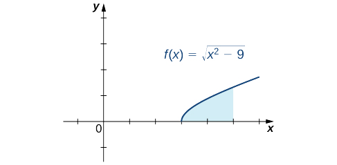
Figure \(\PageIndex{7}\): Calculating the area of the shaded region requires evaluating an integral with a trigonometric substitution.

We can see that the area is \(A= \int ^5_3\sqrt{x^2−9} \, dx\). To evaluate this definite integral, substitute \(x=3\sec \theta \) and \(dx=3\sec \theta \tan \theta \, d \theta \). We must also change the limits of integration. If \(x=3\), then \(3=3\sec \theta \) and hence \( \theta =0\). If \(x=5\), then \( \theta =\sec^{−1}(\frac{5}{3})\). After making these substitutions and simplifying, we have\[ \begin{array}{rclcl}
\text{Area} & = & \displaystyle \int ^5_3 \sqrt{x^2−9} \, dx & & \\[6pt]
& = & \displaystyle \int ^{\sec^{−1}(5/3)}_0 9\tan^2 \theta \sec \theta \, d \theta & & \\[6pt]
& = & \displaystyle \int ^{\sec^{−1}(5/3)}_0 9(\sec^2 \theta −1)\sec \theta \, d \theta & \quad & \left( \text{Pythagorean Identity} \right) \\[6pt]
& = & \displaystyle \int ^{\sec^{−1}(5/3)}_0 9(\sec^3 \theta −\sec \theta )\,d \theta & & \\[6pt]
& = & \left( \dfrac{9}{2} \ln |\sec \theta +\tan \theta | + \dfrac{9}{2} \sec \theta \tan \theta − 9 \ln |\sec \theta +\tan \theta | \right) \bigg|^{\sec^{−1}(5/3)}_0 & & \\[6pt]
& = & \left( \dfrac{9}{2} \sec \theta \tan \theta − \dfrac{9}{2} \ln |\sec \theta +\tan \theta | \right) \bigg|^{\sec^{−1}(5/3)}_0 & & \\[6pt]
& = & \dfrac{9}{2} \cdot \dfrac{5}{3} \cdot \dfrac{4}{3} − \dfrac{9}{2} \ln \left| \dfrac{5}{3}+\dfrac{4}{3} \right| − \left( \dfrac{9}{2} \cdot 1 \cdot 0 − \dfrac{9}{2} \ln |1+0| \right) & & \\[6pt]
& = & 10 - \dfrac{9}{2} \ln 3 & & \\[6pt]
\end{array} \nonumber \]

Checkpoint \(\PageIndex{9}\): Finding an Arc Length

Find the length of the curve \(y=x^2\) over the interval \(\left[0,\frac{1}{2}\right]\).

Answer

\( \frac{1}{4}\left( \sqrt{2} + \ln(\sqrt{2}+1) \right) \)

Reduction Formulas

Evaluating \(\displaystyle \int \sec^n(x)\,dx\) for values of \(n\) where \(n\) is odd requires Integration by Parts. In addition, we must also know the value of \(\displaystyle \int \sec^{n−2}(x)\,dx\) to evaluate \(\displaystyle \int \sec^n(x) \,dx\). The evaluation of \(\displaystyle \int \tan^n(x)\,dx\) also requires being able to integrate \(\displaystyle \int \tan^{n−2}(x)\,dx\). We can derive and apply the following Power Reduction Identities for Integration to simplify the process. These rules allow us to replace the integral of a power of \(\sec(x)\) or \(\tan(x)\) with the integral of a lower power of \(\sec(x)\) or \(\tan(x)\).

Theorem: Power Reduction Identities for \( \int \sec^n(x)\,dx\) and \( \int \tan^n(x)\,dx\)

\[ \int \sec^n(x)\,dx=\dfrac{1}{n−1}\sec^{n−2}(x)\tan(x)+\dfrac{n−2}{n−1} \int \sec^{n−2}(x)\,dx \nonumber \]and\[ \int \tan^n(x)\,dx=\dfrac{1}{n−1}\tan^{n−1}(x) − \int \tan^{n−2}(x)\,dx. \nonumber \]

Note

The Power Reduction Identity for Integrating Powers of Secant may be verified by applying Integration by Parts. The Power Reduction Identity for Integrating Powers of Tangent may be verified by following the strategy outlined for integrating odd powers of \(\tan(x).\)

Example \(\PageIndex{10}\): Revisiting \( \int \sec^3(x)\,dx\)

Apply a reduction formula to evaluate \(\displaystyle \int \sec^3(x)\,dx.\)

Solution

By applying the first reduction formula, we obtain\[\begin{array}{rcl}
\displaystyle \int \sec^3(x)\,dx & = & \dfrac{1}{2}\sec(x)\tan(x)+\dfrac{1}{2} \displaystyle \int \sec(x)\,dx \\[6pt]
& = & \dfrac{1}{2}\sec(x)\tan(x)+\dfrac{1}{2}\ln|\sec(x)+\tan(x)|+C. \\[6pt]
\end{array} \nonumber \]

Example \(\PageIndex{11}\): Using a Power Reduction Identity for Integration

Evaluate \(\displaystyle \int \tan^4(x)\,dx.\)

Solution

Applying the Power Reduction Identity for \( \int \tan^4(x)\,dx\) we have\[\begin{array}{rcl}
\displaystyle \int \tan^4(x)\,dx & = & \dfrac{1}{3}\tan^3(x)− \displaystyle \int \tan^2(x)\,dx\\[6pt]
& = & \dfrac{1}{3}\tan^3(x)−(\tan(x)− \displaystyle \int \tan^0(x)\,dx) \\[6pt]
& = & \dfrac{1}{3}\tan^3(x)−\tan(x)+ \displaystyle \int 1\,dx \\[6pt]
& = & \dfrac{1}{3}\tan^3(x)−\tan(x)+x+C \\[6pt]
\end{array} \nonumber \]

Checkpoint \(\PageIndex{11}\)

Apply the Power Reduction Identity to \(\displaystyle \int \sec^5(x)\,dx.\)

Answer

\(\displaystyle \int \sec^5(x)\,dx=\dfrac{1}{4}\sec^3(x)\tan(x)+\dfrac{3}{4} \int \sec^3(x) \, dx\)

---

Footnotes

¹ The capital, bold letters are purposeful here, we will see why momentarily.

² Note that we put LI at the beginning of the mnemonic; however, we could just as easily have started with IL, since these two types of functions won't appear together in an Integration by Parts problem and they are both terrible choices for \( dv \).

³ I use a \( \boxed{?} \) instead of \( \boxed{\checkmark} \) because having a product of two different types of functions within the integrand is not a guarantee that Integration by Parts will work.

⁴ Another way we could have made our choice for \( u \) and \( dv \) here is to note that, since both \( t^2 \) and \( t e^{t^2} \) are integrable, we switch gears and choose \( u \) to be the factor that will eventually change forms given enough derivatives. This will be \( u = t^2 \) because, after two derivatives, it will become a constant function.

⁵ It turns out that Integration by Parts does not require the integrand to be a product of two different function types. It can be used to integrate compositions of functions and it is sometimes used to integrate single functions!