3.4: Area and Arc Length in Polar Coordinates

Learning Objectives

• Apply the formula for area of a region in polar coordinates.
• Determine the arc length of a polar curve.

In the rectangular coordinate system, the definite integral provides a way to calculate the area under a curve. In particular, if we have a function \(y=f(x)\) defined from \(x=a\) to \(x=b\) where \(f(x)>0\) on this interval, the area between the curve and the x-axis is given by

\[A=\int ^b_af(x)dx. \nonumber\]

This fact, along with the formula for evaluating this integral, is summarized in the Fundamental Theorem of Calculus. Similarly, the arc length of this curve is given by

\[L=\int ^b_a\sqrt{1+(f′(x))^2}dx. \nonumber\]

In this section, we study analogous formulas for area and arc length in the polar coordinate system.

Areas of Regions Bounded by Polar Curves

We have studied the formulas for area under a curve defined in rectangular coordinates and parametrically defined curves. Now we turn our attention to deriving a formula for the area of a region bounded by a polar curve. Recall that the proof of the Fundamental Theorem of Calculus used the concept of a Riemann sum to approximate the area under a curve by using rectangles. For polar curves we use the Riemann sum again, but the rectangles are replaced by sectors of a circle.

Consider a curve defined by the function \(r=f(θ),\) where \(α≤θ≤β.\) Our first step is to partition the interval \([α,β]\) into n equal-width subintervals. The width of each subinterval is given by the formula \(Δθ=(β−α)/n\), and the ith partition point \(θ_i\) is given by the formula \(θ_i=α+iΔθ\). Each partition point \(θ=θ_i\) defines a line with slope \(\tan θ_i\) passing through the pole as represented in the Figure \(\PageIndex{1}\).

Figure \(\PageIndex{1}\): On the polar coordinate plane, a curve is drawn in the first quadrant, and there are rays from the pole that intersect this curve at a regular interval. Every time one of these rays intersects the curve, a perpendicular line is made from the ray to the next ray. The first instance of a ray-curve intersection is labeled \(θ = α\); the last instance is labeled \(θ = β\). The intervening ones are marked \(θ_1\),\(θ_2\), …, \(θ_{n−1}\).

The line segments are connected by arcs of constant radius. This defines sectors whose areas can be calculated by using a geometric formula. The area of each sector is then used to approximate the area between successive line segments. We then sum the areas of the sectors to approximate the total area. This approach gives a Riemann sum approximation for the total area. The formula for the area of a sector of a circle is illustrated in the Figure \(\PageIndex{2}\).

Figure \(\PageIndex{2}\): The area of a sector of a circle is given by \(A=\dfrac{1}{2}θr^2\). The image features a circle with a sector highlighted. The circle's boundary is drawn in black. The sector is outlined by two blue lines radiating from the circle's center to its perimeter, forming an angle marked as theta \((θ)\). The radius of the circle is labeled as \("r"\) along one of these radii.

Recall that the area of a circle is \(A=πr^2\). When measuring angles in radians, 360 degrees is equal to \(2π\) radians. Therefore a fraction of a circle can be measured by the central angle \(θ\). The fraction of the circle is given by \(\dfrac{θ}{2π}\), so the area of the sector is this fraction multiplied by the total area:

\[A=(\dfrac{θ}{2π})πr^2=\dfrac{1}{2}θr^2.\]

Since the radius of a typical sector in Figure \(\PageIndex{1}\) is given by \(r_i=f(θ_i)\), the area of the ith sector is given by

\[A_i=\dfrac{1}{2}(Δθ)(f(θ_i))^2.\]

Therefore a Riemann sum that approximates the area is given by

\[A_n=\sum_{i=1}^nA_i≈\sum_{i=1}^n\dfrac{1}{2}(Δθ)(f(θ_i))^2.\]

We take the limit as \(n→∞\) to get the exact area:

\[A=\lim_{n→∞}A_n=\dfrac{1}{2}\int ^β_α(f(θ))^2dθ.\]

Area of a Region Bounded by a Polar Curve

Suppose \(f\) is continuous and nonnegative on the interval \(α≤θ≤β\) with \(0<β−α≤2π\). The area of the region bounded by the graph of \(r=f(θ)\) between the radial lines \(θ=α\) and \(θ=β\) is

\[\begin{align} A =\dfrac{1}{2}\int ^β_α[f(θ)]^2 dθ \\[4pt] =\dfrac{1}{2}\int ^β_αr^2 dθ. \label{areapolar}\end{align}\]

Example \(\PageIndex{1}\): Finding an Area of a Polar Region

Find the area of one petal of the rose defined by the equation \(r=3\sin(2θ).\)

Solution

The graph of \(r=3\sin (2θ)\) follows.

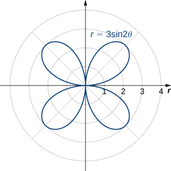
Figure \(\PageIndex{3}\): The graph of \(r=3\sin (2θ).\) A four-petaled rose with furthest point 3 units from the pole occurring at \(π/4\), \(3π/4\), \(5π/4\), and \(7π/4\). The petals are evenly distributed around the center, forming a symmetrical shape.

When \(θ=0\) we have \(r=3\sin(2(0))=0\). The next value for which \(r=0\) is \(θ=π/2\). This can be seen by solving the equation \(3\sin (2θ)=0\) for \(θ\). Therefore the values \(θ=0\) to \(θ=π/2\) trace out the first petal of the rose. To find the area inside this petal, use (Equation \ref{areapolar}) with \(f(θ)=3\sin (2θ), α=0,\) and \(β=π/2\):

\[\begin{align*} A &=\dfrac{1}{2}\int ^β_α[f(θ)]^2dθ \\[4pt] &=\dfrac{1}{2}\int ^{π/2}_0[3\sin (2θ)]^2dθ \\[4pt] &=\dfrac{1}{2}\int ^{π/2}_09\sin^2(2θ)dθ. \end{align*}\]

To evaluate this integral, use the formula \(\sin^2α=(1−\cos (2α))/2\) with \(α=2θ:\)

\[\begin{align*} A &=\dfrac{1}{2}\int ^{π/2}_09\sin^2(2θ)dθ \\[4pt] &=\dfrac{9}{2}\int ^{π/2}_0\dfrac{(1−\cos(4θ))}{2}dθ \\[4pt] &=\dfrac{9}{4}(\int ^{π/2}_01−\cos(4θ)dθ) \\[4pt] &=\dfrac{9}{4}(θ−\dfrac{\sin(4θ)}{4}∣^{π/2}_0 \\[4pt] &=\dfrac{9}{4}(\dfrac{π}{2}−\dfrac{\sin 2π}{4})−\dfrac{9}{4}(0−\dfrac{\sin 4(0)}{4}) \\[4pt] &=\dfrac{9π}{8}\end{align*}\]

Watch the accompanying video for a visual demonstration of this concept.

• Video Length: 2 minutes 3 seconds.
• Context: This video demonstrates how to find the area of one petal of the given equation \(r=3sin(4θ)\).

Exercise \(\PageIndex{1}\)

Find the area inside the cardioid defined by the equation \(r=1−\cos θ\).

Hint

Use (Equation \ref{areapolar}). Be sure to determine the correct limits of integration before evaluating.

Answer

\(A=3π/2\)

Example \(\PageIndex{1}\) involved finding the area inside one curve. We can also use (Equation \ref{areapolar}) to find the area between two polar curves. However, we often need to find the points of intersection of the curves and determine which function defines the outer curve or the inner curve between these two points.

Example \(\PageIndex{2}\): Finding the Area between Two Polar Curves

Find the area outside the cardioid \(r=2+2\sin θ\) and inside the circle \(r=6\sin θ\).

Solution

First draw a graph containing both curves.

Figure \(\PageIndex{4}\): A cardioid with equation \(r=2+2\sin θ\) is graphed, so it has its upper heart part at the pole and the rest of the cardioid is pointed up. There is a circle with radius 6 centered at \((3, π/2)\). The area above the cardioid but below the circle is shaded orange.

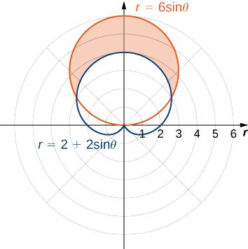
To determine the limits of integration, first find the points of intersection by setting the two functions equal to each other and solving for \(θ\):

\[\begin{align*} 6 \sin θ &=2+2\sin θ \\[4pt] 4\sin θ &=2 \\[4pt] \sin θ &=\dfrac{1}{2} \end{align*}.\]

This gives the solutions \(θ=\dfrac{π}{6}\) and \(θ=\dfrac{5π}{6}\), which are the limits of integration. The circle \(r=3\sin θ\) is the red graph, which is the outer function, and the cardioid \(r=2+2\sin θ\) is the blue graph, which is the inner function. To calculate the area between the curves, start with the area inside the circle between \(θ=\dfrac{π}{6}\) and \(θ=\dfrac{5π}{6}\), then subtract the area inside the cardioid between \(θ=\dfrac{π}{6}\) and \(θ=\dfrac{5π}{6}\):

\(A=\text{circle}−\text{cardioid}\)

\(=\dfrac{1}{2}\int ^{5π/6}_{π/6}[6\sin θ]^2dθ−\dfrac{1}{2}\int ^{5π/6}_{π/6}[2+2\sin θ]^2dθ\)

\(=\dfrac{1}{2}\int ^{5π/6}_{π/6}36\sin^2θ\,dθ−\dfrac{1}{2}\int ^{5π/6}_{π/6}4+8\sin θ+4\sin^2θ\,dθ\)

\(=18\int ^{5π/6}_{π/6}\dfrac{1−\cos(2θ)}{2}dθ−2\int ^{5π/6}_{π/6}1+2\sin θ+\dfrac{1−\cos(2θ)}{2}dθ\)

\(=9[θ−\dfrac{\sin(2θ)}{2}]^{5π/6}_{π/6}−2[\dfrac{3θ}{2}−2\cos θ−\dfrac{\sin(2θ)}{4}]^{5π/6}_{π/6}\)

\(=9(\dfrac{5π}{6}−\dfrac{\sin(10π/6)}{2})−9(\dfrac{π}{6}−\dfrac{\sin(2π/6)}{2})−(3(\dfrac{5π}{6})−4\cos\dfrac{5π}{6}−\dfrac{\sin(10π/6)}{2})+(3(\dfrac{π}{6})−4\cos\dfrac{π}{6}−\dfrac{\sin(2π/6)}{2})\)

\(=4π\).

Exercise \(\PageIndex{2}\)

Find the area inside the circle \(r=4\cos θ\) and outside the circle \(r=2\).

Hint

Use (Equation \ref{areapolar}) and take advantage of symmetry.

Answer

\(A=\dfrac{4π}{3}+2\sqrt{3}\)

In Example \(\PageIndex{2}\) we found the area inside the circle and outside the cardioid by first finding their intersection points. Notice that solving the equation directly for \(θ\) yielded two solutions: \(θ=\dfrac{π}{6}\) and \(θ=\dfrac{5π}{6}\). However, in the graph there are three intersection points. The third intersection point is the pole. The reason why this point did not show up as a solution is because the pole is on both graphs but for different values of \(θ\). For example, for the cardioid we get

\[\begin{align*} 2+2\sin θ =0 \\[4pt] \sin θ =−1 ,\end{align*}.\]

so the values for \(θ\) that solve this equation are \(θ=\dfrac{3π}{2}+2nπ\), where \(n\) is any integer. For the circle we get

\[6\sin θ=0.\]

The solutions to this equation are of the form \(θ=nπ\) for any integer value of \(n\). These two solution sets have no points in common. Regardless of this fact, the curves intersect at the pole. This case must always be taken into consideration.

Arc Length in Polar Curves

Here we derive a formula for the arc length of a curve defined in polar coordinates. In rectangular coordinates, the arc length of a parameterized curve \((x(t),y(t))\) for \(a≤t≤b\) is given by

\[L=\int ^b_a\sqrt{\left(\dfrac{dx}{dt}\right)^2+\left(\dfrac{dy}{dt}\right)^2}dt.\]

In polar coordinates we define the curve by the equation \(r=f(θ)\), where \(α≤θ≤β.\) In order to adapt the arc length formula for a polar curve, we use the equations

\[x=r\cos θ=f(θ)\cos θ\]

and

\[y=r\sin θ=f(θ)\sin θ,\]

and we replace the parameter \(t\) by \(θ\). Then

\[\dfrac{dx}{dθ}=f′(θ)\cos θ−f(θ)\sin θ\]

\[\dfrac{dy}{dθ}=f′(θ)\sin θ+f(θ)\cos θ.\]

We replace \(dt\) by \(dθ\), and the lower and upper limits of integration are \(α\) and \(β\), respectively. Then the arc length formula becomes

\[ \begin{align*} L &=\int ^b_a\sqrt{\left(\dfrac{dx}{dt}\right)^2+\left(\dfrac{dy}{dt}\right)^2}\,dt \\[4pt] &=\int ^β_α\sqrt{\left(\dfrac{dx}{dθ}\right)^2+\left(\dfrac{dy}{dθ}\right)^2}\,dθ \\[4pt] &=\int ^β_α\sqrt{(f′(θ)\cos θ−f(θ)\sin θ)^2+(f′(θ)\sin θ+f(θ)\cos θ)^2}\,dθ \\[4pt] &=\int ^β_α\sqrt{(f′(θ))^2(\cos^2 θ+\sin^2 θ)+(f(θ))^2(\cos^2 θ+\sin^2θ)}\,dθ \\[4pt] &=\int ^β_α\sqrt{(f′(θ))^2+(f(θ))^2}\,dθ \\[4pt] &=\int ^β_α\sqrt{r^2+\left(\dfrac{dr}{dθ}\right)^2}\,dθ \end{align*}\]

Arc Length of a Curve Defined by a Polar Function

Let \(f\) be a function whose derivative is continuous on an interval \(α≤θ≤β\). The length of the graph of \(r=f(θ)\) from \(θ=α\) to \(θ=β\) is

\[ \begin{align} L &=\int ^β_α\sqrt{[f(θ)]^2+[f′(θ)]^2}\,dθ \label{arcpolar1} \\[4pt] &=\int ^β_α\sqrt{r^2+\left(\dfrac{dr}{dθ}\right)^2}\,dθ. \label{arcpolar2} \end{align}\]

Example \(\PageIndex{3}\): Finding the Arc Length of a cardioid

Find the arc length of the cardioid \(r=2+2\cos θ\).

Solution

When \(θ=0,r=2+2\cos 0 =4.\) Furthermore, as \(θ\) goes from \(0\) to \(2π\), the cardioid is traced out exactly once. Therefore these are the limits of integration. Using \(f(θ)=2+2\cos θ, α=0,\) and \(β=2π,\) (Equation \ref{arcpolar1}) becomes

\[\begin{align*} L &=\int ^β_α\sqrt{[f(θ)]^2+[f′(θ)]^2}\,dθ \\[4pt] &=\int ^{2π}_0\sqrt{[2+2\cos θ]^2+[−2\sin θ]^2}\,dθ \\[4pt] &=\int ^{2π}_0\sqrt{4+8\cos θ+4\cos^2θ+4\sin^2θ}\,dθ \\[4pt] &=\int ^{2π}_0\sqrt{4+8\cos θ+4(\cos^2θ+\sin^2θ)}\,dθ \\[4pt] &=\int ^{2π}_0\sqrt{8+8\cos θ}\,dθ \\[4pt] &=2\int ^{2π}_0\sqrt{2+2\cos θ}\,dθ. \end{align*}\]

Next, using the identity \(\cos(2α)=2\cos^2α−1,\) add 1 to both sides and multiply by 2. This gives \(2+2\cos(2α)=4\cos^2α.\) Substituting \(α=θ/2\) gives \(2+2\cos θ=4\cos^2(θ/2)\), so the integral becomes

\[\begin{align*} L &= 2\int ^{2π}_0\sqrt{2+2\cos θ}\,dθ \\[4pt] &=2\int ^{2π}_0\sqrt{4\cos^2(\dfrac{θ}{2})}\,dθ \\[4pt] &=4\int ^{2π}_0∣\cos(\dfrac{θ}{2})∣\,dθ.\end{align*}\]

The absolute value is necessary because the cosine is negative for some values in its domain. To resolve this issue, change the limits from \(0\) to \(π\) and double the answer. This strategy works because cosine is positive between \(0\) and \(\dfrac{π}{2}\). Thus,

\[\begin{align*} L &=4\int ^{2π}_0∣\cos(\dfrac{θ}{2})∣\,dθ \\[4pt] &=8\int ^π_0 \cos(\dfrac{θ}{2})\,dθ \\[4pt] &=8(2\sin(\dfrac{θ}{2})∣^π_0 \\[4pt] &=16\end{align*}\]

Watch the accompanying video for a visual demonstration of this concept.

• Video Length: 1 minute 36 seconds.
• Context: This video demonstrates how to find the arc length of a given polar curve \(r=1+cosθ\),\(0≤θ≤2π\).

Exercise \(\PageIndex{3}\)

Find the total arc length of \(r=3\sin θ\).

Hint

Use (Equation \ref{arcpolar1}). To determine the correct limits, make a table of values.

Answer

\(s=3π\)

Key Concepts

• The area of a region in polar coordinates defined by the equation \(r=f(θ)\) with \(α≤θ≤β\) is given by the integral \(A=\dfrac{1}{2}\int ^β_α[f(θ)]^2dθ\).
• To find the area between two curves in the polar coordinate system, first find the points of intersection, then subtract the corresponding areas.
• The arc length of a polar curve defined by the equation \(r=f(θ)\) with \(α≤θ≤β\) is given by the integral \(L=\int ^β_α\sqrt{[f(θ)]^2+[f′(θ)]^2}dθ=\int ^β_α\sqrt{r^2+(\dfrac{dr}{dθ})^2}dθ\).

Key Equations

• Area of a region bounded by a polar curve \[A=\dfrac{1}{2}\int ^β_α[f(θ)]^2dθ=\dfrac{1}{2}\int ^β_αr^2dθ \nonumber\]
• Arc length of a polar curve \[L=\int ^β_α\sqrt{[f(θ)]^2+[f′(θ)]^2}dθ=\int ^β_α\sqrt{r^2+(\dfrac{dr}{dθ})^2}dθ \nonumber\]

Glossary

Polar Coordinates

A coordinate system where each point on a plane is determined by an angle and a distance from a reference point.

Polar Equation

An equation that expresses the relationship between the radius \(r\) and the angle \(θ\) in polar coordinates.

Area in Polar Coordinates

The area enclosed by a curve in polar coordinates can be found using an integral involving the polar equation.

Arc Length in Polar Coordinates

The length of a curve in polar coordinates can be calculated using an integral involving the polar equation.