5.3E: Exercises for Section 5.3

Exercises 1 - 5 Determining Arc Length

Find the arc length of the curve on the given interval.

1. \(\mathbf r(t)=t^2 \,\mathbf{i}+(2t^2+1)\,\mathbf{j}, \quad 1≤t≤3\)

Answer

\(8\sqrt{5}\) units

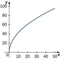
2. \(\mathbf r(t)=t^2 \,\mathbf{i}+14t \,\mathbf{j},\quad 0≤t≤7\). This portion of the graph is shown here:

Figure \(\PageIndex{1}\): The graph of the given vector function is a smooth planar curve. The \(x\) values along the horizontal axis ranges from 0 to 50, and the \(y\) values along the vertical axis ranges from 0 to 100. The curve starts at the origin and increases in a concave down way.

3. \(\mathbf r(t)=⟨t^2+1,4t^3+3⟩, \quad −1≤t≤0\)

Answer

\(\frac{1}{54}(37^{3/2}−1)\) units

4. \(\mathbf r(t)=⟨2 \sin t,5t,2 \cos t⟩,\quad 0≤t≤π\). This portion of the graph is shown here:

Figure \(\PageIndex{2}\): The graph of the given vector function is a smooth space curve. The plot is enclosed within a rectangular box with the horizontal axis ranging from 0 to 2, the vertical axis ranging from -2 to 2, and the depth axis ranging from 0 to 15. The curve goes from the bottom-left back corner, gradually ascending diagonally along a sinusoidal curve through the space, and toward the far-left top corner of the box.

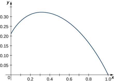
5. \(\mathbf r(t)=\langle e^{−t} \cos t,e^{−t }\sin t \rangle\) over the interval \([0,\frac{π}{2}]\). Here is the portion of the graph on the indicated interval:

Figure \(\PageIndex{3}\): The graph of the given vector function is a smooth planar curve. The \(x\) values along the horizontal axis ranges from \(0\) to approximately \(1\), and the \(y\) values along the vertical axis ranges from \(0\) to approximately \(0.35\). The curve is in the first quadrant, goes from the point \( (1,0) \) to approximately \( (0, 0.21) \). The shape of the curve is concave down and it reaches a local maximum at about \( (0.32, 0.32)\).

6. Set up an integral to represent the arc length from \(t = 0\) to \(t = 2\) along the curve traced out by \(\mathbf r(t) = \langle t, \, t^4\rangle.\) Then use technology to approximate this length to the nearest thousandth of a unit.
7. Find the length of one turn of the helix given by \(\mathbf r(t)= \frac{1}{2} \cos t \,\mathbf{i}+\frac{1}{2} \sin t \,\mathbf{j}+\frac{\sqrt{3}}{2}\,t \,\mathbf{k}\).

Answer

Length \(=2π\) units

8. Find the arc length of the vector-valued function \(\mathbf r(t)=−t \,\mathbf{i}+4t \,\mathbf{j}+3t \,\mathbf{k}\) over \([0,1]\).
9. A particle travels in a circle with the equation of motion \(\mathbf r(t)=3 \cos t \,\mathbf{i}+3 \sin t \,\mathbf{j} +0 \,\mathbf{k}\). Find the distance traveled around the circle by the particle.

Answer

\(6π\) units

10. Set up an integral to find the circumference of the ellipse with the equation \(\mathbf r(t)= \cos t \,\mathbf{i}+2 \sin t \,\mathbf{j}+0\,\mathbf{k}\).
11. Find the length of the curve \(\mathbf r(t)=⟨\sqrt{2}t,\, e^t, \, e^{−t}⟩\) over the interval \(0≤t≤1\). The graph is shown here:

Figure \(\PageIndex{4}\): The graph of the given vector function is a smooth space curve. The plot is enclosed within a rectangular box with the horizontal axis ranging from 0 to 1.5, the vertical axis ranging from 0.4 to 1, and the depth axis ranging from 1 to 2.5. The curve goes from the top-left front corner, quickly descending diagonally, and ending at the bottom-right back corner.

Answer

\(\left(e−\frac{1}{e}\right)\) units

12. Find the length of the curve \(\mathbf r(t)=⟨2 \sin t, \, 5t, \, 2 \cos t⟩\) for \(t∈[−10,10]\).

Exercises 13 - 26 Unit Tangent Vectors and Unit Normal Vectors

13. The position function for a particle is \(\mathbf r(t)=a \cos( ωt) \,\mathbf{i}+b \sin (ωt) \,\mathbf{j}\). Find the unit tangent vector and the unit normal vector at \(t=0\).

Solution:

\(\begin{align*} \mathbf r'(t) &= -aω \sin( ωt) \,\mathbf{i}+bω \cos (ωt) \,\mathbf{j}\\[5pt]
\| \mathbf r'(t) \| &= \sqrt{a^2 ω^2 \sin^2(ωt) +b^2ω^2\cos^2(ωt)} \\[5pt]
\mathbf T(t) &= \dfrac{\mathbf r'(t)}{\| \mathbf r'(t) \| } = \dfrac{-aω \sin( ωt) \,\mathbf{i}+bω \cos (ωt) \,\mathbf{j}}{\sqrt{a^2 ω^2 \sin^2(ωt) +b^2ω^2\cos^2(ωt)}}\\[5pt]
\mathbf T(0) &= \dfrac{bω \,\mathbf{j}}{\sqrt{(bω)^2}} = \dfrac{bω \,\mathbf{j}}{|bω|}\end{align*}\)

If \(bω > 0, \; \mathbf T(0) = \mathbf{j},\) and if \( bω < 0, \; T(0)= -\mathbf{j}\)

Answer

If \(bω > 0, \; \mathbf T(0)= \mathbf{j},\) and if \( bω < 0, \; \mathbf T(0)= -\mathbf{j}\)

If \(a > 0, \; \mathbf N(0)= -\mathbf{i},\) and if \( a < 0, \; \mathbf N(0)= \mathbf{i}\)

14. Given \(\mathbf r(t)=a \cos (ωt) \,\mathbf{i} +b \sin (ωt) \,\mathbf{j}\), find the binormal vector \(\mathbf B(0)\).
15. Given \(\mathbf r(t)=⟨2e^t,e^t \cos t,e^t \sin t⟩\), determine the unit tangent vector \(\mathbf T(t)\).

Answer

\(\begin{align*} \mathbf T(t) &=\left\langle \frac{2}{\sqrt{6}},\, \frac{\cos t− \sin t}{\sqrt{6}}, \, \frac{\cos t+ \sin t}{\sqrt{6}}\right\rangle \\[4pt]
&= \left\langle\frac{\sqrt{6}}{3},\, \frac{\sqrt{6}}{6} (\cos t− \sin t), \, \frac{\sqrt{6}}{6} (\cos t+ \sin t)\right\rangle \end{align*}\)

16. Given \(\mathbf r(t)=⟨2e^t,\, e^t \cos t,\, e^t \sin t⟩\), find the unit tangent vector \(\mathbf T(t)\) evaluated at \(t=0\), \(\mathbf T(0)\).
17. Given \(\mathbf r(t)=⟨2e^t,\, e^t \cos t,\, e^t \sin t⟩\), determine the unit normal vector \(\mathbf N(t)\).

Answer

\(\mathbf N(t)=⟨0,\, -\frac{\sqrt{2}}{2} (\sin t + \cos t), \, \frac{\sqrt{2}}{2} (\cos t- \sin t)⟩\)

18. Given \(\mathbf r(t)=⟨2e^t,\, e^t \cos t,\, e^t \sin t⟩\), find the unit normal vector \(\mathbf N(t)\) evaluated at \(t=0\), \(\mathbf N(0)\).

Answer

\(\mathbf N(0)=⟨0, \;-\frac{\sqrt{2}}{2},\;\frac{\sqrt{2}}{2}⟩\)

19. Given \(\mathbf r(t)=t \,\mathbf{i}+t^2 \,\mathbf{j}+t \,\mathbf{k}\), find the unit tangent vector \(\mathbf T(t)\). The graph is shown here:

Figure \(\PageIndex{5}\): The graph of the given vector function is a smooth space curve. The plot is enclosed within a rectangular box with the horizontal axis ranging from -5 to 5, the vertical axis ranging from -5 to 5, and the depth axis ranging from 0 to 26. The curve goes from the bottom-left back corner, moving forward and up, then back and up, ending at the top-right back corner.

Answer

\(\mathbf T(t)=\dfrac{1}{\sqrt{4t^2+2}}<1,2t,1>\)

20) Find the unit tangent vector \(\mathbf T(t)\) and unit normal vector \(\mathbf N(t)\) at \(t=0\) for the plane curve \(\mathbf r(t)=⟨t^3−4t,5t^2−2⟩\). The graph is shown here:

Figure \(\PageIndex{6}\): The graph of the given vector function is a smooth planar curve. The \(x\) values along the horizontal axis ranges from \(-80\) to approximately \(80\), and the \(y\) values along the vertical axis ranges from \(-20\) to approximately \(140\). The curve is symmetric across the \(y\)-axis, with one narrow region near the origin where the curve intersects itself. As \(x\) moves farther from \(0\) in both positive and negative directions, the curve widens and rises symmetrically along the \(y\)-axis.

21. Find the unit tangent vector \(\mathbf T(t)\) for \(\mathbf r(t)=3t \,\mathbf{i}+5t^2 \,\mathbf{j}+2t \,\mathbf{k}\).

Answer

\(\mathbf T(t)=\dfrac{1}{\sqrt{100t^2+13}}(3 \,\mathbf{i}+10t \,\mathbf{j}+2 \,\mathbf{k})\)

22. Find the principal normal vector to the curve \(\mathbf r(t)= \langle 6 \cos t,6 \sin t \rangle \) at the point determined by \(t=\frac{π}{3}\).
23. Find \(\mathbf T(t)\) for the curve \(\mathbf r(t)=(t^3−4t) \,\mathbf{i}+(5t^2−2) \,\mathbf{j}\).

Answer

\(\mathbf T(t)=\dfrac{1}{\sqrt{9t^4+76t^2+16}}\big((3t^2−4)\,\mathbf{i}+10t \,\mathbf{j}\big)\)

24. Find \(\mathbf N(t)\) for the curve \(\mathbf r(t)=(t^3−4t)\,\mathbf{i}+(5t^2−2)\,\mathbf{j}\).
25. Find the unit tangent vector \(\mathbf T(t)\) for \(\mathbf r(t)= \langle 2 \sin t,\, 5t,\, 2 \cos t \rangle\).

Answer

\(\mathbf T(t)=⟨\frac{2\sqrt{29}}{29}\cos t,\, \frac{5\sqrt{29}}{29},\,−\frac{2\sqrt{29}}{29}\sin t⟩\)

26. Find the unit normal vector \(\mathbf N(t)\) for \(\mathbf r(t)=⟨2\sin t,\,5t,\,2\cos t⟩\).

Answer

\(\mathbf N(t)=⟨−\sin t,\, 0,\, −\cos t⟩\)

Exercises 27 - 29 Arc Length Parameterizations

27. Find the arc-length function \(\mathbf s(t)\) for the line segment given by \(\mathbf r(t)=⟨3−3t,\, 4t⟩\). Then write the arc-length parameterization of \(r\) with \(s\) as the parameter.

Answer

Arc-length function: \(s(t)=5t\); The arc-length parameterization of \(\mathbf r(t)\): \(\mathbf r(s)=\left(3−\dfrac{3s}{5}\right)\,\mathbf{i}+\dfrac{4s}{5}\,\mathbf{j}\)

28. Parameterize the helix \(\mathbf r(t)= \cos t \,\mathbf{i}+ \sin t \,\mathbf{j}+t \,\mathbf{k}\) using the arc-length parameter \(s\), from \(t=0\).
29. Parameterize the curve using the arc-length parameter \(s\), at the point at which \(t=0\) for \(\mathbf r(t)=e^t \sin t \,\mathbf{i} + e^t \cos t \,\mathbf{j}\)

Answer

\(\mathbf r(s)=\left(1+\dfrac{s}{\sqrt{2}}\right) \sin \left( \ln \left(1+ \dfrac{s}{\sqrt{2}}\right)\right)\,\mathbf{i} +\left(1+ \dfrac{s}{\sqrt{2}}\right) \cos \left( \ln \left(1+\dfrac{s}{\sqrt{2}}\right)\right)\,\mathbf{j}\)

Exercises 30 - 50 Curvature and the Osculating Circle

30. Find the curvature of the curve \(\mathbf r(t)=5 \cos t \,\mathbf{i}+4 \sin t \,\mathbf{j}\) at \(t=π/3\). (Note: The graph is an ellipse.)

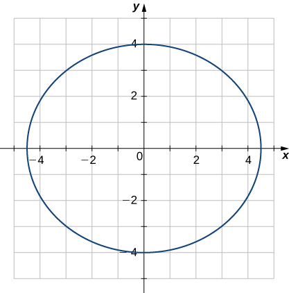
Figure \(\PageIndex{7}\): The graph of the given vector function is an ellipse centered at the origin, with \(x\) values ranging from \(-3.5\) to \(3.5\), and \(y\) values ranging from \(-4\) to \(4\).

31. Find the \(x\)-coordinate at which the curvature of the curve \(y=1/x\) is a maximum value.

Answer

The maximum value of the curvature occurs at \(x=1\).

32. Find the curvature of the curve \(\mathbf r(t)=5 \cos t \,\mathbf{i}+5 \sin t \,\mathbf{j}\). Does the curvature depend upon the parameter \(t\)?
33. Find the curvature \(κ\) for the curve \(y=x−\frac{1}{4}x^2\) at the point \(x=2\).

Answer

\(\frac{1}{2}\)

34. Find the curvature \(κ\) for the curve \(y=\frac{1}{3}x^3\) at the point \(x=1\).
35. Find the curvature \(κ\) of the curve \(\mathbf r(t)=t \,\mathbf{i}+6t^2 \,\mathbf{j}+4t \,\mathbf{k}\). The graph is shown here:

Figure \(\PageIndex{8}\): The graph of the given vector function has a parabolic shape. The curve opens upward and appears symmetric, with its lowest point near the center at the origin. The plot is enclosed within a rectangular box with the horizontal axis ranging from -2 to 2, the vertical axis ranging from 0 to 20, and the depth axis ranging from 8 to -8.

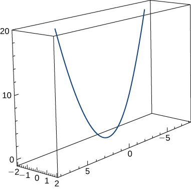
Answer

\(κ≈\dfrac{49.477}{(17+144t^2)^{3/2}}\)

36. Find the curvature of \(\mathbf r(t)=⟨2 \sin t,5t,2 \cos t⟩\).
37. Find the curvature of \(\mathbf r(t)=\sqrt{2}t \,\mathbf{i}+e^t \,\mathbf{j}+e^{−t} \,\mathbf{k}\) at point \(P(0,1,1)\).

Answer

\(\frac{1}{2\sqrt{2}}\)

38. At what point does the curve \(y=e^x\) have maximum curvature?
39. What happens to the curvature as \(x→∞\) for the curve \(y=e^x\)?

Answer

The curvature approaches zero.

40. Find the point of maximum curvature on the curve \(y=\ln x\).
41. Find the equations of the normal plane and the osculating plane of the curve \(\mathbf r(t)=⟨2 \sin (3t),t,2 \cos (3t)⟩\) at point \((0,π,−2)\).

Answer

\(y=6x+π\) and \(x+6y=6π\)

42. Find equations of the osculating circles of the ellipse \(4y^2+9x^2=36\) at the points \((2,0)\) and \((0,3)\).
43. Find the equation for the osculating plane at point \(t=π/4\) on the curve \(\mathbf r(t)=\cos (2t) \,\mathbf{i}+ \sin (2t) \,\mathbf{j}+t\,\mathbf{k}\).

Answer

\(x+2z=\frac{π}{2}\)

44. Find the radius of curvature of \(6y=x^3\) at the point \((2,\frac{4}{3}).\)
45. Find the curvature at each point \((x,y)\) on the hyperbola \(\mathbf r(t)=⟨a \cosh( t),b \sinh (t)⟩\).

Answer

\(\dfrac{a^4b^4}{(b^4x^2+a^4y^2)^{3/2}}\)

46. Calculate the curvature of the circular helix \(\mathbf r(t)=r \sin (t) \,\mathbf{i}+r \cos (t) \,\mathbf{j}+t \,\mathbf{k}\).
47. Find the radius of curvature of \(y= \ln (x+1)\) at point \((2,\ln 3)\).

Answer

\(\frac{10\sqrt{10}}{3}\)

48. Find the radius of curvature of the hyperbola \(xy=1\) at point \((1,1)\).

Exercises 49 - 51

A particle moves along the plane curve \(C\) described by \(\mathbf r(t)=t \,\mathbf{i}+t^2 \,\mathbf{j}\). Use this parameterization to answer the following questions.

49. Find the length of the curve over the interval \([0,2]\).

Answer

\(\frac{1}{4}\big[ 4\sqrt{17} + \ln\left(4+\sqrt{17}\right)\big]\text{ units }\approx 4.64678 \text{ units}\)

50. Find the curvature of the plane curve at \(t=0,1,2\).
51. Describe the curvature as t increases from \(t=0\) to \(t=2\).

Answer

The curvature is decreasing over this interval.

Exercises 52 - 54

The surface of a large cup is formed by revolving the graph of the function \(y=0.25x^{1.6}\) from \(x=0\) to \(x=5\) about the \(y\)-axis (measured in centimeters).

52. [T] Use technology to graph the surface.
53. Find the curvature \(κ\) of the generating curve as a function of \(x\).

Answer

\(κ=\dfrac{30}{x^{2/5}\left(25+4x^{6/5}\right)^{3/2}}\)

Note that initially your answer may be:
\(\dfrac{6}{25x^{2/5}\left(1+\frac{4}{25}x^{6/5}\right)^{3/2}}\)

We can simplify it as follows:
\( \begin{align*} \dfrac{6}{25x^{2/5}\left(1+\frac{4}{25}x^{6/5}\right)^{3/2}} &= \dfrac{6}{25x^{2/5}\big[\frac{1}{25}\left(25+4x^{6/5}\right)\big]^{3/2}}\\[4pt]
&= \dfrac{6}{25x^{2/5}\left(\frac{1}{25}\right)^{3/2}\big[25+4x^{6/5}\big]^{3/2}} \\[4pt]
&= \dfrac{6}{\frac{25}{125}x^{2/5}\big[25+4x^{6/5}\big]^{3/2}} \\[4pt]
&= \dfrac{30}{x^{2/5}\left(25+4x^{6/5}\right)^{3/2}}\end{align*} \)

54. [T] Use technology to graph the curvature function.

Contributors:

• Gilbert Strang (MIT) and Edwin “Jed” Herman (Harvey Mudd) with many contributing authors. This content by OpenStax is licensed with a CC-BY-SA-NC 4.0 license. Download for free at http://cnx.org.

• Paul Seeburger (Monroe Community College) created question 6.