1.5: Applications to Physics

Learning Objectives

• Determine the current for circuit diagram by solving a linear system.
• Determine dimensionless variables by solving a linear system.

Resistor Networks

The tools of linear algebra can be used to study the application of resistor networks. An example of an electrical circuit is below.

Figure \(\PageIndex{1}\) A circuit with a voltage source of 18 volts that forms a closed rectangular path with three resistors and an arrow indicating current flow. The resistors have resistance 2Ω, 4Ω, and 2Ω, as we move clockwise from the voltage source. The current flow, \(I_1\), is counterclockwise.

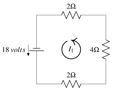
The jagged lines (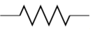) denote resistors and the numbers next to them give their resistance in ohms, written as \(\Omega\). The voltage source () causes the current to flow in the direction from the shorter of the two lines toward the longer (as indicated by the arrow). The current for a circuit is labeled \(I_k\).

In the Figure \(\PageIndex{1}\), the current \(I_1\) has been labeled with an arrow in the counter clockwise direction. This is an entirely arbitrary decision and we could have chosen to label the current in the clockwise direction. With our choice of direction here, we define a positive current to flow in the counter clockwise direction and a negative current to flow in the clockwise direction.

The goal of this section is to use the values of resistors and voltage sources in a circuit to determine the current. An essential theorem for this application is Kirchhoff’s law.

Theorem \(\PageIndex{1}\): Kirchhoff’s Law

The sum of the resistance (\(R\)) times the amps (\(I\)) in the counter clockwise direction around a loop equals the sum of the voltage sources (\(V\)) in the same direction around the loop.

Kirchhoff’s law allows us to set up a system of linear equations and solve for any unknown variables. When setting up this system, it is important to trace the circuit in the counter clockwise direction. If a resistor or voltage source is crossed against this direction, the related term must be given a negative sign.

We will explore this in the next example where we determine the value of the current in the initial diagram.

Example \(\PageIndex{1}\): Solving for Current

Applying Kirchhoff’s Law to the circuit in Figure \(\PageIndex{1}\), determine the value for \(I_1\).

Solution

Begin in the bottom left corner, and trace the circuit in the counter clockwise direction. At the first resistor, multiplying resistance and current gives \(2I_1\). Continuing in this way through all three resistors gives \(2I_1 + 4I_1 + 2 I_1\). This must equal the voltage source in the same direction. Notice that the direction of the voltage source matches the counter clockwise direction specified, so the voltage is positive.

Therefore the equation and solution are given by \[\begin{aligned} 2I_1 + 4I_1 + 2 I_1 &= 18 \\ 8I_1 &= 18 \\ I_1 &= \frac{9}{4} A\end{aligned}\]

Since the answer is positive, this confirms that the current flows counter clockwise.

Example \(\PageIndex{2}\) Solving for Current

Applying Kirchhoff’s Law to the circuit diagram below, determine the value for \(I_1\).

Figure \(\PageIndex{2}\) A circuit with a voltage source of 27 volts that forms a closed rectangular path with four resistors and an arrow indicating current flow. The resistors have resistance 3Ω, 1Ω, 6Ω, and 4Ω, as we move clockwise from the voltage source. The current flow, \(I_1\), is counterclockwise.

Solution

Begin in the top left corner this time, and trace the circuit in the counter clockwise direction. At the first resistor, multiplying resistance and current gives \(4I_1\). Continuing in this way through the four resistors gives \(4I_1 + 6I_1 + 1 I_1 + 3I_1\). This must equal the voltage source in the same direction. Notice that the direction of the voltage source is opposite to the counter clockwise direction, so the voltage is negative.

Therefore the equation and solution are given by \[\begin{aligned} 4I_1 + 6I_1 + 1 I_1 + 3I_1&= -27 \\ 14I_1 &= -27 \\ I_1 &= -\frac{27}{14} A\end{aligned}\]

Since the answer is negative, this tells us that the current flows clockwise.

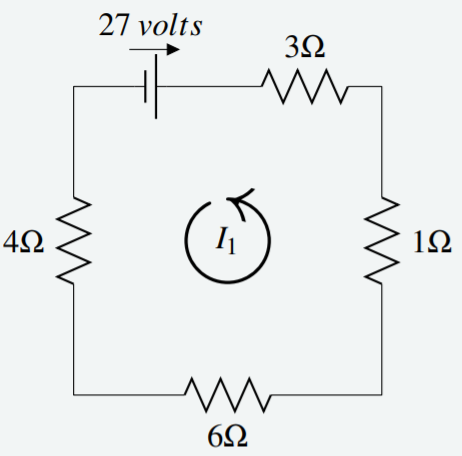
A more complicated example follows. Two of the circuits below may be familiar; they were examined in the examples above. However as they are now part of a larger system of circuits, the answers will differ.

Example \(\PageIndex{3}\): Unknown Currents

The diagram below consists of four circuits. The current (\(I_k\)) in the four circuits is denoted by \(I_{1},I_{2},I_{3},I_{4}\). Using Kirchhoff’s Law, write an equation for each circuit and solve for each current.

Solution

The circuits are given in the following diagram.

Figure \(\PageIndex{3}\) A circuit with multiple interconnected components, including resistors, voltage sources, and current loops. The circuit is arranged in a 2x2 grid, dividing the circuit into 4 squares: Square 1 on the bottom left, Square 2 on the top left, Square 3 on the top right and Square 4 on the bottom right. Square 1 has counterclockwise current flow \(I_1\), with a 23V voltage source with arrow pointing up, and resistors 5Ω along the bottom, 1Ω on the right shared with Square 4, and 2Ω above shared with Square 2. Square 2 has counterclockwise current flow \(I_2\), with an 18V voltage source with arrow pointing down, and resistors 2Ω on the bottom shared with Square 1, 4Ω on the right, shared iwth Square 3, and 2Ω above. Square 3 has counterclockwise current flow \(I_3\), with resistors 4Ω on the left shared with Square 2, 6Ω on the bottom shared with Square 4, 1Ω on the right, 3Ω above, and a 27V voltage source with arrow pointing right. Square 4 has counterclockwise current flow \(I_4\), with resistors 1Ω on the left shared with Square 1, 3Ω below, 2Ω on the right and 6Ω above shared with Square 3.

Starting with the top left circuit, multiply the resistance by the amps and sum the resulting products. Specifically, consider the resistor labeled \(2 \Omega\) that is part of the circuits of \(I_1\) and \(I_2\). Notice that current \(I_2\) runs through this in a positive (counter clockwise) direction, and \(I_1\) runs through in the opposite (negative) direction. The product of resistance and amps is then \(2 (I_2 - I_1) = 2I_2 - 2I_1\). Continue in this way for each resistor, and set the sum of the products equal to the voltage source to write the equation: \[2I_{2}-2I_{1}+4I_{2}-4I_{3}+2I_{2}=18\nonumber \] The above process is used on each of the other three circuits, and the resulting equations are:

Upper right circuit: \[4I_{3} - 4I_{2} + 6I_{3} - 6I_{4} + I_{3} + 3I_{3} = -27\nonumber \] Lower right circuit: \[3I_{4} + 2I_{4} + 6I_{4} - 6I_{3} + I_{4} - I_{1} = 0\nonumber \] Lower left circuit: \[5I_{1}+I_{1}-I_{4}+2I_{1}-2I_{2}=-23\nonumber \]

Notice that the voltage for the upper right and lower left circuits are negative due to the clockwise direction they indicate.

The resulting system of four equations in four unknowns is \[\begin{aligned} 2I_{2}-2I_{1}+4I_{2}-4I_{3}+2I_{2}&=18 \\ 4I_{3} - 4I_{2} + 6I_{3} - 6I_{4} + I_{3} + I_{3} &= -27 \\ 2I_{4} + 3I_{4} + 6I_{4} - 6I_{3} + I_{4} - I_{1} &= 0 \\ 5I_{1}+I_{1}-I_{4}+2I_{1}-2I_{2}&= -23\end{aligned}\] Simplifying and rearranging with variables in order, we have: \[\begin{aligned} -2I_{1}+8I_{2}-4I_{3}&=18 \\ - 4I_{2} + 14I_{3} - 6I_{4} &= -27 \\ -I_{1} - 6I_{3} + 12I_{4} &= 0 \\ 8I_{1}-2I_{2} - I_{4} &= -23\end{aligned}\] The augmented matrix is \[\left[ \begin{array}{rrrr|r} -2 & 8 & -4 & 0 & 18 \\ 0 & -4 & 14 & -6 & -27 \\ -1 & 0 & -6 & 12 & 0 \\ 8 & -2 & 0 & -1 & -23 \end{array} \right]\nonumber \]

The solution to this matrix is \[\begin{aligned} I_{1} &= -3 A\\ I_{2} &= \frac{1}{4} A\\ I_{3} &= -\frac{5}{2} A\\ I_{4} &= -\frac{3}{2} A\end{aligned}\]

This tells us that currents \(I_1, I_3,\) and \(I_4\) travel clockwise while \(I_2\) travels counter clockwise.

Dimensionless Variables

This section shows how solving systems of equations can be used to determine appropriate dimensionless variables. It is only an introduction to this topic and considers a specific example of a simple airplane wing shown below. We assume for simplicity that it is a flat plane at an angle to the wind which is blowing against it with speed \(V\) as shown in Figure \(\PageIndex{4}\).

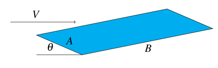
Figure \(\PageIndex{4}\) The airplane, represented as a slanted rectangle with sides \(A\) and \(B\), is slanted to the right. The horizontal arrow on the left, labeled \(V\) and pointing towards the airplane, indicates wind speed. The slanted side of the rectangle, labeled \(A\), makes an angle \(\theta\) with the horizontal, whereas the other side of the rectangle, labeled \(B\), is horizontal.

The angle \(\theta\) is called the angle of incidence, \(B\) is the span of the wing and \(A\) is called the chord. Denote by \(l\) the lift. Then this should depend on various quantities like \(\theta ,V,B,A\) and so forth. Here is a table which indicates various quantities on which it is reasonable to expect \(l\) to depend.

Table \(\PageIndex{1}\) Quantities with corresponding symbol and units

Variable	Symbol	Units
chord	\(A\)	\(m\)
span	\(B\)	\(m\)
angle incidence	\(\theta\)	\(m^0kg^0sec^0\)
speed of wind	\(V\)	\(m sec^{-1}\)
speed of sound	\(V_0\)	\(m sec^{-1}\)
density of air	\(\rho\)	\(kgm^{-3}\)
viscosity	\(\mu\)	\(kg sec^{-1}m^{-1}\)
lift	\(l\)	\(kg sec^{-2}m\)

Here \(m\) denotes meters, \(\sec\) refers to seconds and \(kg\) refers to kilograms. All of these are likely familiar except for \(\mu\), which we will discuss in further detail now.

Viscosity is a measure of how much internal friction is experienced when the fluid moves. It is roughly a measure of how “sticky" the fluid is. Consider a piece of area parallel to the direction of motion of the fluid. To say that the viscosity is large is to say that the tangential force applied to this area must be large in order to achieve a given change in speed of the fluid in a direction normal to the tangential force. Thus \[\mu \left( \text{area}\right) \left( \text{velocity gradient}\right) =\text{ tangential force}\nonumber \] Hence \[\left( \text{units on }\mu \right) m^{2}\left( \frac{m}{\sec m}\right) =kg\sec ^{-2}m\nonumber \] Thus the units on \(\mu\) are \[kg\sec ^{-1}m^{-1}\nonumber \] as claimed above.

Returning to our original discussion, you may think that we would want \[l=f\left( A,B,\theta ,V,V_{0},\rho ,\mu \right)\nonumber \] This is very cumbersome because it depends on seven variables. Also, it is likely that without much care, a change in the units such as going from meters to feet would result in an incorrect value for \(l\). The way to get around this problem is to look for \(l\) as a function of dimensionless variables multiplied by something which has units of force. It is helpful because first of all, you will likely have fewer independent variables and secondly, you could expect the formula to hold independent of the way of specifying length, mass and so forth. One looks for \[l=f\left( g_{1},\cdots ,g_{k}\right) \rho V^{2}AB\nonumber \] where the units on \(\rho V^{2}AB\) are \[\frac{kg}{m^{3}}\left( \frac{m}{\sec }\right) ^{2}m^{2}=\frac{kg\times m}{ \sec ^{2}}\nonumber \] which are the units of force. Each of these \(g_{i}\) is of the form \[A^{x_{1}}B^{x_{2}}\theta ^{x_{3}}V^{x_{4}}V_{0}^{x_{5}}\rho ^{x_{6}}\mu ^{x_{7}} \label{11julye1f}\] and each \(g_{i}\) is independent of the dimensions. That is, this expression must not depend on meters, kilograms, seconds, etc. Thus, placing in the units for each of these quantities, one needs \[m^{x_{1}}m^{x_{2}}\left( m^{x_{4}}\sec ^{-x_{4}}\right) \left( m^{x_{5}}\sec ^{-x_{5}}\right) \left( kgm^{-3}\right) ^{x_{6}}\left( kg\sec ^{-1}m^{-1}\right) ^{x_{7}}=m^{0}kg^{0}\sec ^{0}\nonumber \] Notice that there are no units on \(\theta\) because it is just the radian measure of an angle. Hence its dimensions consist of length divided by length, thus it is dimensionless. Then this leads to the following equations for the \(x_{i}.\)

\[\begin{array}{cc} m: & x_{1}+x_{2}+x_{4}+x_{5}-3x_{6}-x_{7}=0 \\ \sec :\ & -x_{4}-x_{5}-x_{7}=0 \\ kg: & x_{6}+x_{7}=0 \end{array}\nonumber \]

The augmented matrix for this system is

\[\left[ \begin{array}{rrrrrrr|r} 1 & 1 & 0 & 1 & 1 & -3 & -1 & 0 \\ 0 & 0 & 0 & 1 & 1 & 0 & 1 & 0 \\ 0 & 0 & 0 & 0 & 0 & 1 & 1 & 0 \end{array} \right]\nonumber \] The reduced row-echelon form is given by

\[\left[ \begin{array}{rrrrrrr|r} 1 & 1 & 0 & 0 & 0 & 0 & 1 & 0 \\ 0 & 0 & 0 & 1 & 1 & 0 & 1 & 0 \\ 0 & 0 & 0 & 0 & 0 & 1 & 1 & 0 \end{array} \right]\nonumber \] and so the solutions are of the form \[\begin{aligned} x_{1} &= -x_{2}-x_{7} \\ x_{3} &= x_{3} \\ x_{4} &= -x_{5}-x_{7} \\ x_{6} &= -x_{7}\end{aligned}\] Thus, in terms of vectors, the solution is \[\left[ \begin{array}{c} x_{1} \\ x_{2} \\ x_{3} \\ x_{4} \\ x_{5} \\ x_{6} \\ x_{7} \end{array} \right] =\left[ \begin{array}{c} -x_{2}-x_{7} \\ x_{2} \\ x_{3} \\ -x_{5}-x_{7} \\ x_{5} \\ -x_{7} \\ x_{7} \end{array} \right]\nonumber \] Thus the free variables are \(x_{2},x_{3},x_{5},x_{7}.\) By assigning values to these, we can obtain dimensionless variables by placing the values obtained for the \(x_{i}\) in the formula \(\eqref{11julye1f}\). For example, let \(x_{2}=1\) and all the rest of the free variables are 0. This yields \[x_{1}=-1,x_{2}=1,x_{3}=0,x_{4}=0,x_{5}=0,x_{6}=0,x_{7}=0\nonumber \] The dimensionless variable is then \(A^{-1}B^{1}\). This is the ratio between the span and the chord. It is called the aspect ratio, denoted as \(AR\). Next let \(x_{3}=1\) and all others equal zero. This gives for a dimensionless quantity the angle \(\theta\). Next let \(x_{5}=1\) and all others equal zero. This gives \[x_{1}=0,x_{2}=0,x_{3}=0,x_{4}=-1,x_{5}=1,x_{6}=0,x_{7}=0\nonumber \] Then the dimensionless variable is \(V^{-1}V_{0}^{1}.\) However, it is written as \(V/V_{0}\). This is called the Mach number \(\mathcal{M}\).

Finally, let \(x_{7}=1\) and all the other free variables equal 0. Then \[x_{1}=-1,x_{2}=0,x_{3}=0,x_{4}=-1,x_{5}=0,x_{6}=-1,x_{7}=1\nonumber \] then the dimensionless variable which results from this is \(A^{-1}V^{-1}\rho ^{-1}\mu .\) It is customary to write it as \(Re=\left( AV\rho \right) /\mu\). This one is called the Reynold’s number. It is the one which involves viscosity. Thus we would look for \[l=f\left(Re,AR,\theta ,\mathcal{M}\right) kg\times m/\sec ^{2}\nonumber \] This is quite interesting because it is easy to vary \(Re\) by simply adjusting the velocity or \(A\) but it is hard to vary things like \(\mu\) or \( \rho\). Note that all the quantities are easy to adjust. Now this could be used, along with wind tunnel experiments to get a formula for the lift which would be reasonable. You could also consider more variables and more complicated situations in the same way.