1.2: The Dot Product

In this section, we develop an operation called the dot product, which allows us to quantify how much two vectors have in common even when they initially have different directions. The dot product can also help us measure the angle formed by a pair of vectors and the position of a vector relative to the coordinate axes. It even provides a simple test to determine whether two vectors meet at a right angle.

Definition: Dot Product

The dot product of vectors \(\vecs{ u}=⟨u_1,u_2,u_3⟩\) and \(\vecs{ v}=⟨v_1,v_2,v_3⟩\) is given by the sum of the products of the components

\[\vecs{ u}⋅\vecs{ v}=u_1v_1+u_2v_2+u_3v_3 \nonumber \]

Note that if \(u\) and \(v\) are two-dimensional vectors, we calculate the dot product in a similar fashion. Thus, if \(\vecs{ u}=⟨u_1,u_2⟩\) and \(\vecs{ v}=⟨v_1,v_2⟩,\) then

\[\vecs{ u}⋅\vecs{ v}=u_1v_1+u_2v_2 \nonumber \]

When two vectors are combined under addition or subtraction, the result is a vector. When two vectors are combined using the dot product, the result is a scalar.

Example \(\PageIndex{1}\): Calculating Dot Products

(a) Evaluate \(\vecs{u}\cdot \vecs{v}\) for \(\vecs{ u}=⟨3,5,2⟩\) and \(\vecs{ v}=⟨−1,3,0⟩\)

(b) Find the dot product of \(\vecs{ p}=10\hat{\textbf i}−4 \hat{\textbf j}+7 \hat{\textbf k}\) and \(\vecs{ q}=−2\hat{\textbf i}+\hat{\textbf j}+6\hat{\textbf k}\)

(c) Evaluate \(⟨2,9,−1⟩\cdot ⟨−3,1,−4⟩\)

Solution:

(a) \(\vecs{ u}\cdot \vecs{ v} =3(−1)+5(3)+2(0) =12 \)

(b) \(\vecs{ p}\cdot \vecs{ q}=10(−2)+(−4)(1)+(7)(6)=18\)

(c) \(⟨2,9,−1⟩\cdot ⟨−3,1,−4⟩=2(-3)+9(1)+(-1)(-4)=7\)

Like vector addition and subtraction, the dot product has several algebraic properties. We prove three of these properties and leave the rest as exercises.

Properties of the Dot Product

Let \(\vecs{ u}\), \(\vecs{ v}\), and \(\vecs{ w}\) be vectors, and let \(c\) be a scalar.

1. Commutative property \[\vecs{ u}⋅\vecs{ v}=\vecs{ v}⋅\vecs{ u} \nonumber \]
2. Distributive property \[\vecs{ u}⋅(\vecs{ v}+\vecs{ w})=\vecs{ u}⋅\vecs{ v}+\vecs{ u}⋅\vecs{ w} \nonumber \]
3. Associative property \[c(\vecs{ u}⋅\vecs{ v})=(c\vecs{ u})⋅\vecs{ v}=\vecs{ u}⋅(c\vecs{ v}) \nonumber \]
4. Property of magnitude \[\vecs{ v}⋅\vecs{ v}=\|\vecs{ v}\|^2 \nonumber \]

Proof

Let \(\vecs{ u}=⟨u_1,u_2,u_3⟩\) and \(\vecs{ v}=⟨v_1,v_2,v_3⟩.\) Then

\[ \begin{align*} \vecs{ u}⋅\vecs{ v} &=⟨u_1,u_2,u_3⟩⋅⟨v_1,v_2,v_3⟩ \\[4pt] &=u_1v_1+u_2v_2+u_3v_3 \\[4pt] &= v_1u_1+v_2u_2+v_3u_3 \\[4pt] &= ⟨v_1,v_2,v_3⟩⋅⟨u_1,u_2,u_3⟩ \\[4pt] &=\vecs{ v}⋅\vecs{ u}\end{align*}\]

The associative property looks like the associative property for real-number multiplication, but pay close attention to the difference between scalar and vector objects:

\[ \begin{align*} c(\vecs{ u}⋅\vecs{ v}) &=c(u_1v_1+u_2v_2+u_3v_3) \\[4pt] &=c(u_1v_1)+c(u_2v_2)+c(u_3v_3) \\[4pt] &=(cu_1)v_1+(cu_2)v_2+(cu_3)v_3 \\[4pt] &=⟨cu_1,cu_2,cu_3⟩⋅⟨v_1,v_2,v_3⟩ \\[4pt] &=c⟨u_1,u_2,u_3⟩⋅⟨v_1,v_2,v_3⟩ \\[4pt] &=(c\vecs{ u})⋅\vecs{ v}\end{align*}\]

The proof that \(c(\vecs{ u}⋅\vecs{ v})=\vecs{ u}⋅(c\vecs{ v})\) is similar.

The fourth property shows the relationship between the magnitude of a vector and its dot product with itself:

\[ \begin{align*} \vecs{ v}⋅\vecs{ v} &=⟨v_1,v_2,v_3⟩⋅⟨v_1,v_2,v_3⟩\\[4pt] &=(v_1)^2+(v_2)^2+(v_3)^2 \\[4pt] &=\left[\sqrt{(v_1)^2+(v_2)^2+(v_3)^2}\right]^2 \\[4pt] &=\|\vecs{ v}\|^2\end{align*}\]

Note that the definition of the dot product yields \(\vecs{ 0}⋅\vecs{ v}=0.\) By property iv. if \(\vecs{ v}⋅\vecs{ v}=0,\) then \(\vecs{ v}=\vecs{ 0}.\)

Example \(\PageIndex{2}\): Using Properties of the Dot Product

Let \(\vecs{ a}=⟨1,2,−3⟩\), \(\vecs{ b}=⟨0,2,4⟩\), and \( \vecs{ c} =⟨5,−1,3⟩\).

Find each of the following products.

(a) \(( \vecs{ a} ⋅ \vecs{ b}) \vecs{ c} \)

(b) \(\vecs{ a}⋅(2\vecs{ c})\)

(c) \(\|\vecs{ b}\|^2\)

Solution

(a) Note that this expression asks for the scalar multiple of \(\vecs{ c}\) by \(\vecs{ a}⋅\vecs{ b}\):

\[ \begin{align*} (\vecs{ a}⋅\vecs{ b})\vecs{ c} &=(⟨1,2,−3⟩⋅⟨0,2,4⟩)⟨5,−1,3⟩ \\[4pt] &=(1(0)+2(2)+(−3)(4))⟨5,−1,3⟩ \\[4pt] &=−8⟨5,−1,3⟩ \\[4pt] &= ⟨−40,8,−24⟩\end{align*}\]

(b) This expression is a dot product of vector \(\vecs{ a}\) and scalar multiple 2\(\vecs{ c}\):

\[ \begin{align*} \vecs{ a}⋅(2\vecs{ c}) &=2(\vecs{ a}⋅\vecs{ c}) \\[4pt] &=2(⟨1,2,−3⟩⋅⟨5,−1,3⟩) \\[4pt] &=2(1(5)+2(−1)+(−3)(3)) \\[4pt] &=2(−6)=−12\end{align*}\]

(c) Simplifying this expression is a straightforward application of the dot product:

\[ \begin{align*} \|\vecs{ b}\|^2 &=\vecs{ b}⋅\vecs{ b} \\[4pt] &=⟨0,2,4⟩⋅⟨0,2,4⟩\\[4pt] &=0^2+2^2+4^2\\[4pt] &=0+4+16\\[4pt] &=20\end{align*}\]

When two nonzero vectors are placed in standard position, whether in two dimensions or three dimensions, they form an angle between them. The dot product provides a way to find the measure of this angle. This property is a result of the fact that we can express the dot product in terms of the cosine of the angle formed by two vectors.

Figure \(\PageIndex{1}\): Let \(θ\) be the angle between two nonzero vectors \(\vecs{ u}\) and \(\vecs{ v}\) such that \(0≤θ≤π\).

Evaluating a Dot Product

The dot product of two vectors is the product of the magnitude of each vector and the cosine of the angle between them:

\[\vecs{ u}⋅\vecs{ v}=‖\vecs{ u}‖‖\vecs{ v}‖\cos (θ) \nonumber \]

Proof

Place vectors \(\vecs{ u}\) and \(\vecs{ v}\) in standard position and consider the vector \(\vecs{ v}−\vecs{ u}\) pictured below. These three vectors form a triangle with side lengths \(‖\vecs{ u}‖,‖\vecs{ v}‖\), and \(‖\vecs{ v}−\vecs{ u}‖\).

Figure \(\PageIndex{2}\): The lengths of the sides of the triangle are given by the magnitudes of the vectors that form the triangle.

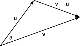
Recall from trigonometry that the law of cosines describes the relationship among the side lengths of the triangle and the angle \(θ\). Applying the law of cosines here gives

\[‖\vecs{ v}−\vecs{ u}‖^2=‖\vecs{ u}‖^2+‖\vecs{ v}‖^2−2‖\vecs{ u}‖‖\vecs{ v}‖\cos (θ) \nonumber \]

The dot product provides a way to rewrite the left side of this equation:

\[ \begin{align*} ‖\vecs{ v}−\vecs{ u}‖^2 &=(\vecs{ v}−\vecs{ u})⋅(\vecs{ v}−\vecs{ u}) \\[4pt] &=(\vecs{ v}−\vecs{ u})⋅\vecs{ v}−(\vecs{ v}−\vecs{ u})⋅\vecs{ u} \\[4pt] &=\vecs{ v}⋅\vecs{ v}−\vecs{ u}⋅\vecs{ v}−\vecs{ v}⋅\vecs{ u}+\vecs{ u}⋅\vecs{ u} \\[4pt] &=\vecs{ v}⋅\vecs{ v}−\vecs{ u}⋅\vecs{ v}−\vecs{ u}⋅\vecs{ v}+\vecs{ u}⋅\vecs{ u} \\[4pt] &=‖\vecs{ v}‖^2−2\vecs{ u}⋅\vecs{ v}+‖\vecs{ u}‖^2\end{align*}\]

Substituting into the law of cosines yields

\[ \begin{align*} ‖\vecs{ v}−\vecs{ u}‖^2 &=‖\vecs{ u}‖^2+‖\vecs{ v}‖^2−2‖\vecs{ u}‖‖\vecs{ v}‖\cos (θ) \\[4pt] ‖\vecs{ v}‖^2−2\vecs{ u}⋅\vecs{ v}+‖\vecs{ u}‖^2 &= ‖\vecs{ u}‖^2+‖\vecs{ v}‖^2−2‖\vecs{ u}‖‖\vecs{ v}‖\cos (θ) \\[4pt] −2\vecs{ u}⋅\vecs{ v} &=−2‖\vecs{ u}‖‖\vecs{ v}‖\cos (θ) \\[4pt] \vecs{ u}⋅\vecs{ v} &=‖\vecs{ u}‖‖\vecs{ v}‖\cos (θ) \end{align*}\]

We can use the dot product to find the measure of the angle between two nonzero vectors by rearranging this equation to solve for the cosine of the angle:

\[\cos (θ)=\dfrac{\vecs{ u}⋅\vecs{ v}}{‖\vecs{ u}‖‖\vecs{ v}‖} \nonumber \]

Using this equation, we can find the cosine of the angle between two nonzero vectors. Since we are considering the smallest angle between the vectors, we assume \(0°≤θ≤180°\) (or \(0≤θ≤π\) if we are working in radians). The inverse cosine is unique over this range, so we are then able to determine the angle \(θ\).

Example \(\PageIndex{3}\): Finding the Angle between Two Vectors

Find the measure of the angle between each pair of vectors.

(a) \(\mathbf{\hat i} + \mathbf{\hat j} + \mathbf{\hat k}\) and \(2\mathbf{\hat i} – \mathbf{\hat j} – 3\mathbf{\hat k}\)

(b) \(⟨2,5,6⟩\) and \(⟨−2,−4,4⟩\)

(c) \(\vecs{ a}=⟨1,1,1⟩\) and \(\vecs{ b}=⟨2\sqrt{3}+\sqrt{2},2\sqrt{3}+\sqrt{2},2\sqrt{3}-2\sqrt{2}⟩\)

Solution

(a) We know that:

\[ \begin{align*} \cos (θ) &=\dfrac{(\mathbf{\hat i}+\mathbf{\hat j}+\mathbf{\hat k})⋅(2\mathbf{\hat i}−\mathbf{\hat j}−3\mathbf{\hat k})}{∥\mathbf{\hat i}+\mathbf{\hat j}+\mathbf{\hat k}∥⋅∥2\mathbf{\hat i}−\mathbf{\hat j}−3\mathbf{\hat k}∥} \\[4pt] &=\dfrac{1(2)+(1)(−1)+(1)(−3)}{\sqrt{1^2+1^2+1^2}\sqrt{2^2+(−1)^2+(−3)^2}} \\[4pt] &=\dfrac{−2}{\sqrt{3}\sqrt{14}} =\dfrac{−2}{\sqrt{42}} \end{align*}\]

Therefore, \(θ=\cos^{-1}\left(\dfrac{−2}{\sqrt{42}}\right)\) radians.

(b) Once more:

\[ \begin{align*} \cos (θ) &=\dfrac{⟨2,5,6⟩⋅⟨−2,−4,4⟩}{∥⟨2,5,6⟩∥⋅∥⟨−2,−4,4⟩∥} \\[4pt] &=\dfrac{2(−2)+(5)(−4)+(6)(4)}{\sqrt{2^2+5^2+6^2}\sqrt{(−2)^2+(−4)^2+4^2}} \\[4pt] &=\dfrac{0}{\sqrt{65}\sqrt{36}}=0\end{align*}\]

Now, \(\cos (θ)=0\) and \(0≤θ≤π\), so \(θ=\dfrac{\pi}{2}\) radians.

(c) Again:

\[ \begin{align*} \cos (θ) &=\dfrac{⟨1,1,1⟩⋅⟨2\sqrt{3}+\sqrt{2},2\sqrt{3}+\sqrt{2},2\sqrt{3}-2\sqrt{2}⟩}{∥⟨1,1,1⟩∥⋅∥⟨2\sqrt{3}+\sqrt{2},2\sqrt{3}+\sqrt{2},2\sqrt{3}-2\sqrt{2}⟩∥} \\[4pt] &=\dfrac{1(2\sqrt{3}+\sqrt{2})+1(2\sqrt{3}+\sqrt{2})+1(2\sqrt{3}-2\sqrt{2})}{\sqrt{1^2+1^2+1^2}\sqrt{(2\sqrt{3}+\sqrt{2})^2+(2\sqrt{3}+\sqrt{2})^2+(2\sqrt{3}-2\sqrt{2})^2}} \\[4pt] &=\dfrac{6\sqrt{3}}{\sqrt{3}\sqrt{48}}=\dfrac{\sqrt{3}}{2}\end{align*}\]

Therefore, \(θ=\cos^{-1}\left(\dfrac{\sqrt{3}}{2}\right)=\dfrac{\pi}{6}\) radians.

The angle between two vectors can be acute \((0<\cos (θ)<1),\) obtuse \((−1<\cos (θ)<0)\), or straight \((\cos (θ)=−1)\). If \(\cos (θ)=1\), then both vectors have the same direction. If \(\cos (θ)=0\), then the vectors, when placed in standard position, form a right angle. We can formalize this result into a theorem regarding orthogonal (perpendicular) vectors.

Figure \(\PageIndex{3}\): (a) An acute angle has \(0<\cos (θ)<1\)
(b) An obtuse angle has \(−1<\cos (θ)<0\)
(c) A straight line has \(\cos (θ)=−1\)
(d) If the vectors have the same direction, \(\cos (θ)=1\)
(e) If the vectors are orthogonal (perpendicular), \(\cos (θ)=0\)

Orthogonal Vectors

The nonzero vectors \(\vecs{u}\) and \(\vecs{v}\) are orthogonal vectors if and only if \(\vecs{u}⋅\vecs{v}=0.\)

Proof

Let \(\vecs{u}\) and \(\vecs{v}\) be nonzero vectors, and let \(θ\) denote the angle between them. First, assume \(\vecs{u}⋅\vecs{v}=0.\)Then

\[‖\vecs{u}‖‖\vecs{v}‖\cos (θ)=0 \nonumber \]

However, \(‖\vecs{u}‖≠0\) and \(‖\vecs{v}‖≠0,\) so we must have \(\cos (θ)=0\). Hence, \(θ=90°\), and the vectors are orthogonal.

Now assume \(\vecs{u}\) and \(\vecs{v}\) are orthogonal. Then \(θ=90°\) and we have

\[ \begin{align*} \vecs{u}⋅\vecs{v} &=‖\vecs{ u}‖‖\vecs{ v}‖\cos θ \\[4pt] &=‖\vecs{ u}‖‖\vecs{ v}‖\cos (90°) \\[4pt] &=‖\vecs{ u}‖‖\vecs{ v}‖(0) \\[4pt] &=0 \end{align*}\]

The terms orthogonal, perpendicular, and normal each indicate that mathematical objects are intersecting at right angles. The use of each term is determined mainly by its context. We say that vectors are orthogonal and lines are perpendicular. The term normal is used most often when measuring the angle made with a plane or other surface.

Example \(\PageIndex{4}\): Identifying Orthogonal Vectors

Determine whether \(\vecs{p}=⟨1,0,5⟩\) and \(\vecs{q}=⟨10,3,−2⟩\) are orthogonal vectors.

Solution

Using the definition, we need only check the dot product of the vectors:

\[ \vecs{ p}⋅\vecs{ q}=1(10)+(0)(3)+(5)(−2)=10+0−10=0 \nonumber \]

Because \(\vecs{p}⋅\vecs{q}=0,\) the vectors are orthogonal.

Example \(\PageIndex{5}\)

For which value(s) of \(x\) is \(\vecs{ p}=⟨2,8,−1⟩\) orthogonal to \(\vecs{ q}=⟨x,−1,2⟩\)?

Solution

We calculate the dot product of the vectors:

\[ \vecs{ p}⋅\vecs{ q}=2(x)+8(-1)+(-1)(2)=2x-10 \nonumber \]

Setting this equal to zero gives \(2x-10=0 \longrightarrow x=5\) as our only solution.

As we have seen, addition combines two vectors to create a resultant vector. But what if we are given a vector and we need to find its component parts? We use vector projections to perform the opposite process; they can break down a vector into its components. The magnitude of a vector projection is a scalar projection. For example, if a child is pulling the handle of a wagon at a 55° angle, we can use projections to determine how much of the force on the handle is actually moving the wagon forward. We return to this example and learn how to solve it after we see how to calculate projections.

Figure \(\PageIndex{4}\): When a child pulls a wagon, only the horizontal component of the force propels the wagon forward.

Definition: Vector and Projection

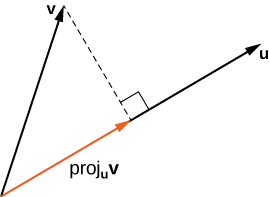
The vector projection of \(\vecs{ v}\) onto \(\vecs{ u}\) is the vector labeled \(\text{proj}_\vecs{ u}\vecs{ v}\) below. It has the same initial point as \(\vecs{ u}\) and \(\vecs{ v}\) and the same direction as \(\vecs{ u}\), and represents the component of \(\vecs{ v}\) that acts in the direction of \(\vecs{ u}\). If \(θ\) represents the angle between \(\vecs{ u}\) and \(\vecs{ v}\), then, by properties of triangles, we know the length of \(\text{proj}_\vecs{ u}\vecs{ v}\) is \(\|\text{proj}_\vecs{ u}\vecs{ v}\|=‖\vecs{ v}‖\cos (θ).\) When expressing \(\cos (θ)\) in terms of the dot product, this becomes

\[ \|\text{proj}_\vecs{ u}\vecs{ v}\|=‖\vecs v‖\cos (θ)=‖\vecs{ v}‖\left(\dfrac{\vecs{ u}⋅\vecs{ v}}{‖\vecs{ u}‖‖\vecs{ v}‖}\right)=\dfrac{\vecs{ u}⋅\vecs{ v}}{‖\vecs{ u}‖} \nonumber \]

We now multiply by a unit vector in the direction of \(\vecs{ u}\) to get \(\text{proj}_\vecs{ u}\vecs{ v}\):

\[\text{proj}_\vecs{ u}\vecs{ v}=\dfrac{\vecs{ u}⋅\vecs{ v}}{‖\vecs{ u}‖}\left(\dfrac{1}{‖\vecs{ u}‖}\vecs{ u}\right)=\dfrac{\vecs{ u}⋅\vecs{ v}}{‖\vecs{ u}‖^2}\vecs{ u} \nonumber \]

The length of this vector is also known as the scalar projection of \(\vecs{ v}\) onto \(\vecs{ u}\) and is denoted by

\[\|\text{proj}_\vecs{ u}\vecs{ v}\|=\text{comp}_\vecs{ u}\vecs{ v}=\dfrac{|\vecs{ u}⋅\vecs{ v}|}{‖\vecs{ u}‖} \nonumber \]

Figure \(\PageIndex{5}\): The projection of \(\vecs{ v}\) onto \(\vecs{ u}\) shows the component of vector \(\vecs{ v}\) in the direction of \(\vecs{ u}\).

Example \(\PageIndex{6}\): Finding Projections

Find the projection of \(\vecs{ v}\) onto \(\vecs{ u}\).

(a) \(\vecs{v}=⟨3,5,1⟩\) and \(\vecs{u}=⟨−1,4,3⟩\)

(b) \(\vecs{v}=3\mathbf{\hat i}−2\mathbf{\hat j}\) and \(\vecs{u}=\mathbf{\hat i}+6\mathbf{\hat j}\)

Solution

(a) Substitute the components of \(\vecs{ v}\) and \(\vecs{ u}\) into the formula for the projection:

\[\begin{align*} \text{proj}_\vecs{ u}\vecs{ v} &=\dfrac{\vecs{ u}⋅\vecs{ v}}{‖\vecs{ u}‖^2}\vecs{ u} \\[4pt] &=\dfrac{⟨−1,4,3⟩⋅⟨3,5,1⟩}{∥⟨−1,4,3⟩∥^2}⟨−1,4,3⟩ \\[4pt] &=\dfrac{−3+20+3}{(−1)^2+4^2+3^2}⟨−1,4,3⟩ \\[4pt] &=\dfrac{20}{26}⟨−1,4,3⟩ \\[4pt] &=\left\langle −\dfrac{10}{13},\dfrac{40}{13},\dfrac{30}{13}\right\rangle \end{align*}\]

(b) To find the two-dimensional projection, simply adapt the formula to the two-dimensional case:

\[\begin{align*} \text{proj}_\vecs{ u}\vecs{ v} &=\dfrac{\vecs{ u}⋅\vecs{ v}}{‖\vecs{ u}‖^2}\vecs{ u} \\[4pt] &=\dfrac{(\mathbf{\hat i}+6\mathbf{\hat j})⋅(3\mathbf{\hat i}−2\mathbf{\hat j})}{∥\mathbf{\hat i}+6\mathbf{\hat j}∥^2}(\mathbf{\hat i}+6\mathbf{\hat j}) \\[4pt] &= \dfrac{1(3)+6(−2)}{1^2+6^2}(\mathbf{\hat i}+6\mathbf{\hat j}) \\[4pt] &= −\dfrac{9}{37}(\mathbf{\hat i}+6\mathbf{\hat j}) \\[4pt] &= −\dfrac{9}{37}\mathbf{\hat i}−\dfrac{54}{37}\mathbf{\hat j}\end{align*}\]

Sometimes it is useful to decompose vectors—that is, to break a vector apart into a sum. This process is called the resolution or decomposition of a vector into components. Projections allow us to identify two orthogonal vectors having a desired sum. For example, let \(\vecs{ v}=⟨6,−4⟩\) and let \(\vecs{ u}=⟨3,1⟩.\) We want to decompose the vector \(\vecs{ v}\) into orthogonal components such that one of the component vectors has the same direction as \(\vecs{ u}\).

We first find the component that has the same direction as \(\vecs{ u}\) by projecting \(\vecs{ v}\) onto \(\vecs{ u}\). Let \(\vecs{ p}=\text{proj}_\vecs{ u}\vecs{ v}\). Then, we have

\[\begin{align*}\vecs{ p} =\dfrac{\vecs{ u}⋅\vecs{ v}}{‖\vecs{ u}‖^2}\vecs{ u} \\[4pt] = \dfrac{18−4}{9+1}\vecs{ u} \\[4pt] = \dfrac{7}{5}\vecs{ u}=\dfrac{7}{5}⟨3,1⟩=\left\langle \dfrac{21}{5},\dfrac{7}{5}\right\rangle \end{align*}\]

Now consider the vector \(\vecs{ q}=\vecs{ v}−\vecs{ p}.\) We have

\[\begin{align*} \vecs{ q} =\vecs{ v}−\vecs{ p} \\[4pt] = ⟨6,−4⟩−\left\langle \dfrac{21}{5},\dfrac{7}{5}\right\rangle \\[4pt] =\left\langle \dfrac{9}{5},−\dfrac{27}{5}\right\rangle \end{align*}\]

Clearly, by the way we defined \(\vecs{ q}\), we have \(\vecs{ v}=\vecs{ q}+\vecs{ p},\) and

\[\begin{align*}\vecs{ q}⋅\vecs{ p} =\left\langle \dfrac{9}{5},−\dfrac{27}{5}\right\rangle \cdot \left\langle \dfrac{21}{5},\dfrac{7}{5}\right\rangle \\[4pt] = \dfrac{9(21)}{25}+−\dfrac{27(7)}{25} \\[4pt] = \dfrac{189}{25}−\dfrac{189}{25}=0 \end{align*}\]

Therefore, \(\vecs{ q}\) and \(\vecs{ p}\) are orthogonal.

Example \(\PageIndex{7}\): Resolving Vectors into Components

Express \(\vecs{ v}=⟨8,−3,−3⟩\) as a sum of orthogonal vectors such that one of the vectors has the same direction as \(\vecs{ u}=⟨2,3,2⟩.\)

Solution

Let \(\vecs{ p}\) represent the projection of \(\vecs{ v}\) onto \(\vecs{ u}\):

\[ \begin{align*} \vecs{ p} &=\text{proj}_\vecs{ u}\vecs{ v} \\[4pt] &=\dfrac{\vecs{ u}⋅\vecs{ v}}{‖\vecs{ u}‖^2}\vecs{ u} \\[4pt] &=\dfrac{⟨2,3,2⟩⋅⟨8,−3,−3⟩}{∥⟨2,3,2⟩∥^2}⟨2,3,2⟩ \\[4pt] &=\dfrac{16−9−6}{2^2+3^2+2^2}⟨2,3,2⟩ \\[4pt] &=\dfrac{1}{17}⟨2,3,2⟩ \\[4pt] &=\left\langle \dfrac{2}{17},\dfrac{3}{17},\dfrac{2}{17}\right\rangle \end{align*} \nonumber \]

Then,

\[ \begin{align*} \vecs{ q} &=\vecs{ v}−\vecs{ p}=⟨8,−3,−3⟩−\left\langle \dfrac{2}{17},\dfrac{3}{17},\dfrac{2}{17}\right\rangle\\[4pt] &=\left\langle \dfrac{134}{17},−\dfrac{54}{17},−\dfrac{53}{17}\right\rangle \end{align*} \nonumber \]

To check our work, we can use the dot product to verify that \(\vecs{ p}\) and \(\vecs{ q}\) are orthogonal vectors:

\[ \begin{align*}\vecs{ p}⋅\vecs{ q}&=\left\langle \dfrac{2}{17},\dfrac{3}{17},\dfrac{2}{17}\right\rangle \cdot \left\langle \dfrac{134}{17},−\dfrac{54}{17},−\dfrac{53}{17} \right\rangle\\[4pt] &=\dfrac{268}{289}−\dfrac{162}{289}−\dfrac{106}{289}=0 \end{align*} \nonumber \]

Then,

\[\vecs{ v}=\vecs{ p}+\vecs{ q}=\left\langle \dfrac{2}{17},\dfrac{3}{17},\dfrac{2}{17} \right\rangle +\left\langle \dfrac{134}{17},−\dfrac{54}{17},−\dfrac{53}{17}\right\rangle \nonumber \]

Now that we understand dot products, we can see how to apply them to real-life situations. The most common application of the dot product of two vectors is in the calculation of work.

From physics, we know that work is done when an object is moved by a force. When the force is constant and applied in the same direction the object moves, then we define the work done as the product of the force and the distance the object travels: \(W=Fd\). Now imagine the direction of the force is different from the direction of motion, as with the example of a child pulling a wagon. To find the work done, we need to multiply the component of the force that acts in the direction of the motion by the magnitude of the displacement. The dot product allows us to do just that. If we represent an applied force by a vector \(\vecs{ F}\) and the displacement of an object by a vector \(\vecs{ s}\), then the work done by the force is the dot product of \(\vecs{ F}\) and \(\vecs{ s}\).

Definition: Constant Force

When a constant force is applied to an object so the object moves in a straight line from point \(P\) to point \(Q\), the work \(W\) done by the force \(\vecs{ F}\), acting at an angle θ from the line of motion, is given by

\[W=\vecs{ F}⋅\vecd{PQ}=∥\vecs{ F}∥∥\vecd{PQ}∥\cos (θ) \nonumber \]

Let’s revisit the problem of the child’s wagon introduced earlier. Suppose a child is pulling a wagon with a force having a magnitude of 8 lb on the handle at an angle of 55°. If the child pulls the wagon 50 ft, find the work done by the force.

Figure \(\PageIndex{6}\): The horizontal component of the force is the projection of \(\vecs{ F}\) onto the positive \(x\)-axis.

We have

\[W=∥\vecs{ F}∥∥\vecd{PQ}∥\cos (θ)=(8\, \text{lb})\, (50 \, \text{ft.})\,\cos(55°)≈229\,\text{ft⋅lb.} \nonumber \]

In U.S. standard units, we measure the magnitude of force \(∥\vecs{ F}∥\) in pounds. The magnitude of the displacement vector \(∥\vecd{PQ}∥\) tells us how far the object moved, and it is measured in feet. The customary unit of measure for work, then, is the foot-pound. One foot-pound is the amount of work required to move an object weighing 1 lb a distance of 1 ft straight up. In the metric system, the unit of measure for force is the newton (N), and the unit of measure of magnitude for work is a newton-meter (N·m), or a joule (J).

Example \(\PageIndex{8}\): Calculating Work

A conveyor belt generates a force \(\vecs{ F}=5\mathbf{\hat i}−3\mathbf{\hat j}+\mathbf{\hat k}\) that moves a suitcase from point \((1,1,1)\) to point \((9,4,7)\) along a straight line. Find the work done by the conveyor belt. The distance is measured in meters and the force is measured in newtons.

Solution

The displacement vector \(\vecd{PQ}\) has initial point \((1,1,1)\) and terminal point \((9,4,7)\):

\[\vecd{PQ}=⟨9−1,4−1,7−1⟩=⟨8,3,6⟩=8\mathbf{\hat i}+3\mathbf{\hat j}+6\mathbf{\hat k} \nonumber \]

Work is the dot product of force and displacement:

\[\begin{align*} W &=\vecs{ F}⋅\vecd{PQ} \\[4pt] &= (5\mathbf{\hat i}−3\mathbf{\hat j}+\mathbf{\hat k})⋅(8\mathbf{\hat i}+3\mathbf{\hat j}+6\mathbf{\hat k}) \\[4pt] &= 5(8)+(−3)(3)+1(6) \\[4pt] &=37\,\text{N⋅m} \\[4pt] &= 37\,\text{J} \end{align*}\]