8.2: Fourier Series I

In Example 8.1.4 and Exercises 8.1.4-8.1.22 we saw that the eigenfunctions of Problem 5 are orthogonal on \([-L,L]\) and the eigenfunctions of Problems 1–4 are orthogonal on \([0,L]\). In this section and the next we introduce some series expansions in terms of these eigenfunctions. We’ll use these expansions to solve partial differential equations in Chapter 9.

Theorem \(\PageIndex{1}\)

Suppose the functions \(\phi_1,\) \(\phi_2,\) \(\phi_3,\) …\(,\) are orthogonal on \([a,b]\) and

\[\label{eq:11.2.1} \int_a^b\phi_n^2(x)\,dx\ne0,\quad n=1,2,3,\dots.\]

Let \(c_1,\) \(c_2,\) \(c_3,\)…be constants such that the partial sums \(f_N(x)=\sum_{m=1}^N c_m\phi_m(x)\) satisfy the inequalities

\[|f_N(x)|\le M,\quad a\le x\le b,\quad N=1,2,3,\dots\nonumber \]

for some constant \(M<\infty.\) Suppose also that the series

\[\label{eq:11.2.2} f(x)=\sum_{m=1}^\infty c_m\phi_m(x)\]

converges and is integrable on \([a,b]\). Then

\[\label{eq:11.2.3} c_n={\int_a^bf(x)\phi_n(x)\,dx\over\int_a^b\phi_n^2(x)\,dx},\quad n=1,2,3,\dots.\]

Proof

Multiplying Equation \ref{eq:11.2.2} by \(\phi_n\) and integrating yields

\[\label{eq:11.2.4} \int_a^b f(x)\phi_n(x)\,dx=\int_a^b \phi_n(x)\left(\sum_{m=1}^\infty c_m\phi_m(x)\right)\,dx.\]

It can be shown that the boundedness of the partial sums \(\{f_N\}_{N=1}^\infty\) and the integrability of \(f\) allow us to interchange the operations of integration and summation on the right of Equation \ref{eq:11.2.4}, and rewrite Equation \ref{eq:11.2.4} as

\[\label{eq:11.2.5} \int_a^b f(x)\phi_n(x)\,dx=\sum_{m=1}^\infty c_m \int_a^b\phi_n(x) \phi_m(x)\,dx.\]

(This isn’t easy to prove.) Since

\[\int_a^b\phi_n(x)\phi_m(x)\,dx=0\quad \text{if} \quad m\ne n,\nonumber \]

Equation \ref{eq:11.2.5} reduces to

\[\int_a^bf(x) \phi_n(x)\,dx=c_n\int_a^b\phi_n^2(x)\,dx.\nonumber \]

Now Equation \ref{eq:11.2.1} implies Equation \ref{eq:11.2.3}.

Theorem \(\PageIndex{1}\) motivates the next definition.

Theorem \(\PageIndex{2}\)

Suppose \(\phi_1,\) \(\phi_2\), …, \(\phi_n\),…are orthogonal on \([a,b]\) and \(\int_a^b\phi_n^2(x)\,dx\ne0\), \(n=1\), \(2\), \(3\), …. Let \(f\) be integrable on \([a,b],\) and define

\[\label{eq:11.2.6} c_n={\int_a^bf(x)\phi_n(x)\,dx\over\int_a^b\phi_n^2(x)\,dx},\quad n=1,2,3,\dots.\]

Then the infinite series \(\sum_{n=1}^\infty c_n\phi_n(x)\) is called the Fourier expansion of \(f\) in terms of the orthogonal set \(\{\phi_n\}_{n=1}^\infty\), and \(c_1\), \(c_2\), …, \(c_n\), … are called the Fourier coefficients of \(f\) with respect to \(\{\phi_n\}_{n=1}^\infty\). We indicate the relationship between \(f\) and its Fourier expansion by

\[\label{eq:11.2.7} f(x)\sim\sum_{n=1}^\infty c_n\phi_n(x),\quad a\le x\le b.\]

You may wonder why we don’t write

\[f(x)=\sum_{n=1}^\infty c_n\phi_n(x),\quad a\le x\le b,\nonumber \]

rather than Equation \ref{eq:11.2.7}. Unfortunately, this isn’t always true. The series on the right may diverge for some or all values of \(x\) in \([a,b]\), or it may converge to \(f(x)\) for some values of \(x\) and not for others. So, for now, we’ll just think of the series as being associated with \(f\) because of the definition of the coefficients \(\{c_n\}\), and we’ll indicate this association informally as in Equation \ref{eq:11.2.7}.

Fourier Series

We’ll now study Fourier expansions in terms of the eigenfunctions

\[1,\, \cos{\pi x\over L},\, \sin{\pi x\over L}, \, \cos{2\pi x\over L}, \, \sin{2\pi x\over L},\dots, \cos{n\pi x\over L}, \, \sin{n\pi x\over L},\dots.\nonumber \]

of Problem 5. If \(f\) is integrable on \([-L,L]\), its Fourier expansion in terms of these functions is called the Fourier series of \(f\) on \([-L,L]\). Since

\[\int_{-L}^L 1^2\,dx=2L,\nonumber \]

\[\int_{-L}^L\cos^2{n\pi x\over L}\,dx = \left.{1\over2}\int_{-L}^L\left(1+\cos{2n\pi x\over L}\right)\,dx= {1\over2}\left(x+{L\over2n\pi}\sin{2n\pi x\over L}\right) \right|_{-L}^{L}=L,\nonumber \]

and

\[\int_{-L}^L\sin^2{n\pi x\over L}\,dx = \left. {1\over2}\int_{-L}^L\left(1-\cos{2n\pi x\over L}\right)\,dx= {1\over2}\left(x-{L\over2n\pi}\sin{2n\pi x\over L}\right), \right|_{-L}^{L}=L,\nonumber \]

we see from Equation \ref{eq:11.2.6} that the Fourier series of \(f\) on \([-L,L]\) is

\[a_0+\sum_{n=1}^\infty \left(a_n\cos{n\pi x\over L}+b_n\sin{n\pi x\over L}\right),\nonumber \]

where

\[a_0={1\over 2L}\int_{-L}^L f(x)\,dx,\nonumber \]

\[a_n= {1\over L}\int_{-L}^L f(x)\cos{n\pi x\over L}\,dx,\quad \text{and} \quad b_n={1\over L}\int_{-L}^L f(x)\sin{n\pi x\over L}\,dx,\,n\ge1.\nonumber \]

Note that \(a_0\) is the average value of \(f\) on \([-L,L]\), while \(a_n\) and \(b_n\) (for \(n\ge1\)) are twice the average values of

\[f(x)\cos{n\pi x\over L}\quad\mbox{ and }\quad f(x)\sin{n\pi x\over L}\nonumber \]

on \([-L,L]\), respectively.

Convergence of Fourier Series

The question of convergence of Fourier series for arbitrary integrable functions is beyond the scope of this book. However, we can state a theorem that settles this question for most functions that arise in applications.

Theorem \(\PageIndex{3}\)

A function \(f\) is said to be piecewise smooth on \([a,b]\) if:

1. \(f\) has at most finitely many points of discontinuity in \((a,b)\);
2. \(f'\) exists and is continuous except possibly at finitely many points in \((a,b)\);
3. \(f(x_0+)=\lim_{x\to x_0+}f(x)\) and \(f'(x_0+)=\lim_{x\to x_0+}f'(x)\) exist if \(a\le x_0<b\);
4. \(f(x_0-)=\lim_{x\to x_0-}f(x)\) and \(f'(x_0-)=\lim_{x\to x_0-}f'(x)\) exist if \(a< x_0\le b\).

Since \(f\) and \(f'\) are required to be continuous at all but finitely many points in \([a,b]\), \(f(x_0+)=f(x_0-)\) and \(f'(x_0+)=f'(x_0-)\) for all but finitely many values of \(x_0\) in \((a,b)\). Recall from Section 8.1 that \(f\) is said to have a jump discontinuity at \(x_0\) if \(f(x_0+)\ne f(x_0-)\).

The next theorem gives sufficient conditions for convergence of a Fourier series. The proof is beyond the scope of this book.

Theorem \(\PageIndex{4}\)

If \(f\) is a piecewise smooth on \([-L,L]\), then the Fourier series

\[\label{eq:11.2.8}F(x)=a_{0}+\sum_{n=1}^{\infty}\left(a_{n}\cos\frac{n\pi x}{L}+b_{n}\sin\frac{n\pi x}{L} \right)\] of \(f\) on \([-L,L]\) converges for all \(x\) in \([-L,L]\); moreover,

\[F(x)=\left\{\begin{array}{cc}{f(x)}&{if\:-L<x<L\:and\:f\:is\:continuous\:at\:x}\\{\frac{f(x-)+f(x+)}{2}}&{if\:-L<x<L\:and\:f\:is\:discontinuous\:at\:x}\\{\frac{f(-L+)+f(L-)}{2}}&{if\:x=L\:or\:x=-L}\end{array} \right.\nonumber\]

Since \(f(x+)=f(x-)\) if \(f\) is continuous at \(x\), we can also say that

\[F(x)=\left\{\begin{array}{cc}{\frac{f(x+)+f(x-)}{2}}&{if\:-L<x<L}\\{\frac{f(L-)+f(-L+)}{2}}&{if\:x=\pm L}\end{array} \right.\nonumber\]

Note that \(F\) is itself piecewise smooth on \([-L,L]\), and \(F(x)=f(x)\) at all points in the open interval \((-L,L)\) where \(f\) is continuous. Since the series in Equation \ref{eq:11.2.8} converges to \(F(x)\) for all \(x\) in \([-L,L]\), you may be tempted to infer that the error

\[E_N(x)= \left|F(x)-a_0-\sum_{n=1}^N\left(a_n\cos{n\pi x\over L}+b_n\sin{n\pi x\over L}\right)\right|\nonumber \]

can be made as small as we please for all \(x\) in \([-L,L]\) by choosing \(N\) sufficiently large. However, this isn’t true if \(f\) has a discontinuity somewhere in \((-L,L)\), or if \(f(-L+)\ne f(L-)\). Here’s the situation in this case.

If \(f\) has a jump discontinuity at a point \(\alpha\) in \((-L,L)\), there will be sequences of points \(\{u_N\}\) and \(\{v_N\}\) in \((-L,\alpha)\) and \((\alpha,L)\), respectively, such that

\[\lim _{N\to\infty}u_{N}=\lim _{N\to\infty}v_{N}=\alpha \nonumber \]

and

\[E_N(u_N)\approx .09|f(\alpha-)-f(\alpha+)| \quad \text{and} \quad E_N(v_N)\approx .09|f(\alpha-)-f(\alpha+)|.\nonumber \]

Thus, the maximum value of the error \(E_N(x)\) near \(\alpha\) does not approach zero as \(N\to\infty\), but just occurs closer and closer to \((\)and on both sides of \()\) \(\alpha\), and is essentially independent of \(N\).

If \(f(-L+)\ne f(L-)\), then there will be sequences of points \(\{u_N\}\) and \(\{v_N\}\) in \((-L,L)\) such that

\[\lim_{N\to\infty}u_N=-L,\quad \lim_{N\to\infty}v_N=L,\nonumber \]

\[E_N(u_N)\approx .09|f(-L+)-f(L-)| \quad \text{and} \quad E_N(v_N)\approx .09|f(-L+)-f(L-)|.\nonumber \]

This is the Gibbs phenomenon. Having been alerted to it, you may see it in Figures \(\PageIndex{2}\) - \(\PageIndex{4}\), below; however, we’ll give a specific example at the end of this section.

Example \(\PageIndex{1}\)

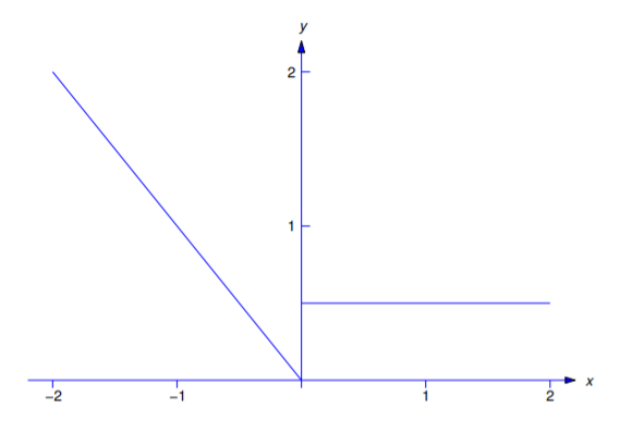
Find the Fourier series of the piecewise smooth function

\[f(x)= \left\{\begin{array}{rlr} -x,&-2< x<0, \\{1\over2},&\phantom{-}0<x<2 \end{array}\right.\nonumber \]

on \([-2,2]\) (Figure \(\PageIndex{1}\)). Determine the sum of the Fourier series for \(-2\le x\le 2\).

Figure \(\PageIndex{1}\)

Solution

Note that wen’t bothered to define \(f(-2)\), \(f(0)\), and \(f(2)\). No matter how they may be defined, \(f\) is piecewise smooth on \([-2,2]\), and the coefficients in the Fourier series

\[F(x)=a_0+\sum_{n=1}^\infty\left(a_n\cos{n\pi x\over2}+b_n\sin{n\pi x\over2}\right)\nonumber \]

are not affected by them. In any case, Theorem \(\PageIndex{4}\) implies that \(F(x)=f(x)\) in \((-2,0)\) and \((0,2)\), where \(f\) is continuous, while

\[F(-2)=F(2)={f(-2+)+f(2-)\over2}= {1\over2}\left(2+{1\over2}\right)={5\over4}\nonumber \]

and

\[F(0)={f(0-)+f(0+)\over2}={1\over2}\left(0+{1\over2}\right)={1\over4}.\nonumber \]

To summarize,

\[F(x)= \left\{\begin{array}{rl} {5\over4},&\phantom{-}x=-2\\ -x,&-2<x<0,\\ {1\over4},&\phantom{-}x=0,\\ {1\over2},&\phantom{-}0<x<2,\\ {5\over4},&\phantom{-}x=2. \end{array}\right.\nonumber \]

We compute the Fourier coefficients as follows:

\[a_0={1\over4}\int_{-2}^2f(x)\,dx={1\over4}\left[\int_{-2}^0(-x)\,dx +\int_0^2{1\over2}\,dx\right] ={3\over4}.\nonumber \]

If \(n\ge1\), then

\[\begin{aligned} a_n&={1\over2}\int_{-2}^2f(x)\cos{n\pi x\over2}\,dx={1\over2}\left[\int_{-2}^0(-x)\cos{n\pi x\over2}\,dx +\int_0^2{1\over2}\cos{n\pi x\over2}\,dx\right]\\&={2\over n^2\pi^2}(\cos n\pi-1),\end{aligned}\nonumber \]

and

\[\begin{aligned} b_n&={1\over2}\int_{-2}^2f(x)\sin{n\pi x\over2}\,dx={1\over2}\left[\int_{-2}^0(-x)\sin{n\pi x\over2}\,dx +\int_0^2{1\over2}\sin{n\pi x\over2}\,dx\right]\\ &={1\over2n\pi}(1+3\cos n\pi).\end{aligned}\nonumber \]

Therefore

\[F(x)={3\over4}+{2\over\pi^2}\sum_{n=1}^\infty{\cos n\pi-1\over n^2}\cos{n\pi x\over2}+{1\over2\pi}\sum_{n=1}^\infty{1+3\cos n\pi\over n}\sin{n\pi x\over2}.\nonumber \]

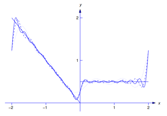
Figure \(\PageIndex{2}\) shows how the partial sum

\[F_m(x)={3\over4}+{2\over\pi^2}\sum_{n=1}^m{\cos n\pi-1\over n^2}\cos{n\pi x\over2}+{1\over2\pi}\sum_{n=1}^m{1+3\cos n\pi\over n}\sin{n\pi x\over2}\nonumber \]

approximates \(f(x)\) for \(m=5\) (dotted curve), \(m=10\) (dashed curve), and \(m=15\) (solid curve).

Figure \(\PageIndex{2}\)

Even and Odd Functions

Computing the Fourier coefficients of a function \(f\) can be tedious; however, the computation can often be simplified by exploiting symmetries in \(f\) or some of its terms. To focus on this, we recall some concepts that you studied in calculus. Let \(u\) and \(v\) be defined on \([-L,L]\) and suppose that

\[u(-x)=u(x)\quad\mbox{ and }\quad v(-x)=-v(x),\quad -L\le x\le L.\nonumber \]

Then we say that \(u\) is an even function and \(v\) is an odd function. Note that:

• The product of two even functions is even.
• The product of two odd functions is even.
• The product of an even function and an odd function is odd.

Example \(\PageIndex{2}\)

The functions \(u(x)=\cos \omega x\) and \(u(x)=x^2\) are even, while \(v(x)=\sin \omega x\) and \(v(x)=x^3\) are odd. The function \(w(x)=e^x\) is neither even nor odd.

You learned parts (a) and (b) of the next theorem in calculus, and the other parts follow from them (Exercise 11.2.1).

Theorem \(\PageIndex{5}\)

Suppose \(u\) is even and \(v\) is odd on \([-L,L].\) Then\(:\)

1. \(\int_{-L}^L u(x)\,dx=2\int_0^Lu(x) \,dx,\)
2. \(\int_{-L}^L v(x)\,dx=0,\)
3. \(\int_{-L}^L u(x)\cos{n\pi x\over L}\,dx=2\int_0^Lu(x)\cos{n\pi x\over L} \,dx,\)
4. \(\int_{-L}^L v(x)\sin{n\pi x\over L}\,dx= 2\int_0^L v(x)\sin{n\pi x\over L}\,dx,\)
5. \(\int_{-L}^L u(x)\sin{n\pi x\over L}\,dx=0\)
6. \(\int_{-L}^L v(x)\cos{n\pi x\over L}\,dx=0.\)

Example \(\PageIndex{3}\)

Find the Fourier series of \(f(x)=x^2-x\) on \([-2,2]\), and determine its sum for \(-2\le x\le 2\).

Solution

Since \(L=2\),

\[F(x)=a_0+\sum_{n=1}^\infty\left(a_n\cos{n\pi x\over2}+b_n\sin{n\pi x\over2}\right)\nonumber \]

where

\[\label{eq:11.2.9} a_0={1\over4}\int_{-2}^2(x^2-x)\,dx,\]

\[\label{eq:11.2.10} a_n={1\over2}\int_{-2}^2(x^2-x)\cos{n\pi x\over2}\,dx,\quad n=1,2,3,\dots,\]

and

\[\label{eq:11.2.11} b_n={1\over2}\int_{-2}^2(x^2-x)\sin{n\pi x\over2}\,dx,\quad n=1,2,3,\dots.\]

We simplify the evaluation of these integrals by using Theorem [thmtype:11.2.5} with \(u(x)=x^2\) and \(v(x)=x\); thus, from Equation \ref{eq:11.2.9},

\[a_0=\left.{1\over2}\int_0^2x^2\,dx={x^3\over6}\right| _{0}^{2}={4\over3}.\nonumber \]

From Equation \ref{eq:11.2.10},

\[\begin{aligned} a_n&=\int_0^2x^2\cos{n\pi x\over2}\,dx= \left.{2\over n\pi}\left[x^2\sin{n\pi x\over2}\right| _{0}^{2}- 2\int_0^2x\sin{n\pi x\over2}\,dx\right]\\ &=\left. {8\over n^2\pi^2}\left[x\cos{n\pi x\over2}\right| _{0}^{2}- \int_0^2\cos{n\pi x\over2}\,dx\right]\\ &=\left.{8\over n^2\pi^2}\left[2\cos n\pi-{2\over n\pi}\sin{n\pi x\over2}\right|_{0}^{2}\right] =(-1)^n{16\over n^2\pi^2}.\end{aligned}\nonumber \]

From Equation \ref{eq:11.2.11},

\[\begin{aligned} b_n&=-\int_0^2x\sin{n\pi x\over2}\,dx =\left. {2\over n\pi}\left[x\cos{n\pi x\over2}\right|_{0}^{2}- \int_0^2\cos{n\pi x\over2}\,dx\right]\\ &=\left.{2\over n\pi}\left[2\cos n\pi-{2\over n\pi}\sin{n\pi x\over2}\right|_{0}^{2} \right]=(-1)^n{4\over n\pi}.\end{aligned}\nonumber \]

Therefore

\[F(x)={4\over3}+{16\over\pi^2}\sum_{n=1}^\infty{(-1)^n\over n^2} \cos{n\pi x\over2}+{4\over\pi}\sum_{n=1}^\infty {(-1)^n\over n}\sin{n\pi x\over2}.\nonumber \]

Theorem \(\PageIndex{4}\) implies that

\[F(x)= \left\{\begin{array}{cl} 4,&\phantom{-}x=-2,\\ x^2-x,&-2<x<2,\\4,&\phantom{-}x=2. \end{array}\right.\nonumber \]

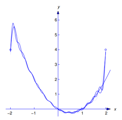
Figure \(\PageIndex{3}\) shows how the partial sum

\[F_m(x)={4\over3}+{16\over\pi^2}\sum_{n=1}^m{(-1)^n\over n^2} \cos{n\pi x\over2}+{4\over\pi}\sum_{n=1}^m {(-1)^n\over n}\sin{n\pi x\over2}\nonumber \]

approximates \(f(x)\) for \(m=5\) (dotted curve), \(m=10\) (dashed curve), and \(m=15\) (solid curve).

Figure \(\PageIndex{3}\): Approximation of \(f(x)=x^{2}-x\) by partial sums of its Fourier series on \([-2,2]\)

Theorem \(\PageIndex{5}\) ilmplies the next theorem follows.

Theorem \(\PageIndex{6}\)

Suppose \(f\) is integrable on \([-L,L].\)

1. If \(f\) is even\(,\) the Fourier series of \(f\) on \([-L,L]\) is \[F(x)=a_0+\sum_{n=1}^\infty a_n\cos{n\pi x\over L},\nonumber \] where \[a_0={1\over L}\int_0^Lf(x) \,dx \quad \text{and} \quad a_n={2\over L}\int_0^L f(x)\cos{n\pi x\over L}\,dx,\quad n\ge1.\nonumber \]
2. If \(f\) is odd\(,\) the Fourier series of \(f\) on \([-L,L]\) is \[F(x)= \sum_{n=1}^\infty b_n \sin{n\pi x\over L},\nonumber \] where \[b_n={2\over L}\int_0^L f(x)\sin{n\pi x\over L}\,dx.\nonumber \]

Example \(\PageIndex{4}\)

Find the Fourier series of \(f(x)=x\) on \([-\pi,\pi]\), and determine its sum for \(-\pi\le x\le \pi\).

Solution

Since \(f\) is odd and \(L=\pi\),

\[F(x)=\sum_{n=1}^\infty b_n\sin nx\nonumber \]

where

\[\begin{aligned} b_n&={2\over\pi}\int_0^\pi x\sin nx\,dx=\left. -{2\over n\pi}\left[x\cos nx\right|_{0}^{\pi }-\int_0^\pi\cos nx\,dx\right]\\ &=\left.-{2\over n}\cos n\pi+{2\over n^2\pi}\sin nx\right|_{0}^{\pi }=(-1)^{n+1} {2\over n}.\end{aligned}\nonumber \]

Therefore

\[F(x)=-2\sum_{n=1}^\infty{(-1)^n\over n}\sin nx.\nonumber \]

Theorem \(\PageIndex{4}\) implies that

\[F(x)= \left\{\begin{array}{cl} 0,&\phantom{-}x=-\pi,\\ x,&-\pi<x<\pi,\\0,&\phantom{-}x=\pi. \end{array}\right.\nonumber \]

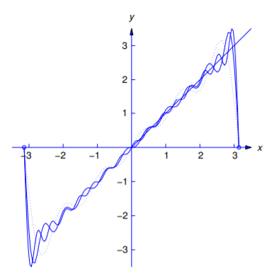
Figure \(\PageIndex{4}\) shows how the partial sum

\[F_m(x)=-2\sum_{n=1}^m{(-1)^n\over n}\sin nx\nonumber \]

approximates \(f(x)\) for \(m=5\) (dotted curve), \(m=10\) (dashed curve), and \(m=15\) (solid curve).

Figure \(\PageIndex{4}\): Approximation of \(f(x)=x\) by partial sums of its Fourier series on \([-\pi ,\pi ]\)

Example \(\PageIndex{5}\)

Find the Fourier series of \(f(x)=|x|\) on \([-\pi,\pi]\) and determine its sum for
\(-\pi\le x\le\pi\).

Solution:

Since \(f\) is even and \(L=\pi\),

\[F(x)=a_0+\sum_{n=1}^\infty a_n\cos nx.\nonumber \]

Since \(f(x)=x\) if \(x\ge0\),

\[a_0=\left. {1\over\pi}\int_0^\pi x\,dx={x^2\over2\pi}\right|_{0}^{\pi }={\pi\over2}\nonumber \]

and, if \(n\ge1\),

\[\begin{aligned} a_n&=\left.{2\over\pi}\int_0^\pi x\cos nx\,dx={2\over n\pi}\left[x\sin nx\right|_{0}^{\pi }-\int_0^\pi\sin nx\,dx\right]\\ &=\left.{2\over n^2\pi}\cos nx\right|_{0}^{\pi }=\frac{2}{n^2\pi}(\cos n\pi-1)={2\over n^2\pi}[(-1)^n-1].\end{aligned}\nonumber \]

Therefore

\[\label{eq:11.2.12} F(x)={\pi\over2}+{2\over\pi}\sum_{n=0}{(-1)^n-1\over n^2}\cos nx.\]

However, since

\[(-1)^n-1= \left\{\begin{array}{rl} 0&\mbox{ if }n=2m,\\ -2&\mbox{ if }n=2m+1, \end{array}\right.\nonumber \]

the terms in Equation \ref{eq:11.2.12} for which \(n=2m\) are all zeros. Therefore we only to include the terms for which \(n=2m+1\); that is, we can rewrite Equation \ref{eq:11.2.12} as

\[F(x)={\pi\over2}-{4\over\pi}\sum_{m=0}^\infty {1\over(2m+1)^2} \cos(2m+1)x.\nonumber \]

However, since the name of the index of summation doesn’t matter, we prefer to replace \(m\) by \(n\), and write

\[F(x)={\pi\over2}-{4\over\pi}\sum_{n=0}^\infty {1\over(2n+1)^2} \cos(2n+1)x.\nonumber \]

Since \(|x|\) is continuous for all \(x\) and \(|-\pi|=|\pi|\), Theorem \(\PageIndex{4}\) implies that \(F(x)=|x|\) for all \(x\) in \([-\pi,\pi]\).

Example \(\PageIndex{6}\)

Find the Fourier series of \(f(x)=x(x^2-L^2)\) on \([-L,L]\), and determine its sum for \(-L\le x\le L\).

Solution:

Since \(f\) is odd,

\[F(x)=\sum_{n=1}^\infty b_n\sin\frac{n\pi x}{L},\nonumber \]

where

\[\begin{aligned} b_n&={2\over L}\int_0^Lx(x^2-L^2)\sin{n\pi x\over L}\,dx\\ &\left.=-{2\over n\pi}\left[x(x^2-L^2)\cos{n\pi x\over L}\right|_{0}^{L}- \int_0^L (3x^2-L^2)\cos{n\pi x\over L}\,dx\right]\\ &=\left.{2L\over n^2\pi^2}\left[(3x^2-L^2)\sin{n\pi x\over L}\right|_{0}^{L}-6 \int_0^Lx\sin{n\pi x\over L}\,dx\right]\\ &=\left.{12L^2\over n^3\pi^3}\left[x\cos{n\pi x\over L}\right|_{0}^{L}- \int_0^L\cos{n\pi x\over L}\,dx\right] =(-1)^n{12L^3\over n^3\pi^3}.\end{aligned}\nonumber \]

Therefore

\[F(x)={12L^3\over\pi^3}\sum_{n=1}^\infty{(-1)^n\over n^3}\sin{n\pi x\over L}.\nonumber \]

Theorem \(\PageIndex{4}\) implies that \(F(x)=x(x^2-L^2)\) for all \(x\) in \([-L,L]\).

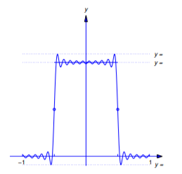
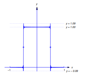
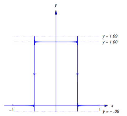
Example \(\PageIndex{7}\) Gibbs Phenomenon

The Fourier series of

\[f(x)=\left\{\begin{array}{cl} 0,&-1<x<-{1\over2},\\ 1,&-{1\over2}<x<{1\over2},\\ 0,&\phantom{-}{1\over2}<x<1 \end{array}\right.\nonumber \]

on \([-1,1]\) is

\[F(x)={1\over2}+{2\over\pi}\sum_{n=1}^\infty {(-1)^{n-1}\over2n-1}\cos(2n-1)\pi x.\nonumber \]

(Verify.) According to Theorem \(\PageIndex{4}\),

\[F(x)=\left\{\begin{array}{cl} 0,&-1\le x<-{1\over2},\\ {1\over2},& x=-{1\over2},\\ 1,&-{1\over2}<x<{1\over2},\\ {1\over2},& x={1\over2},\\ 0,&{1\over2}<x\le 1; \end{array}\right.\nonumber \]

thus, \(F\) (as well as \(f\)) has unit jump discontinuities at \(x=\pm\frac{1}{2}\). Figures \(\PageIndex{5}\)-\(\PageIndex{7}\) show the graphs of \(y=f(x)\) and

\[y=F_{2N-1}(x)=\frac{1}{2}+ {2\over\pi}\sum_{n=1}^N {(-1)^{n-1}\over2n-1}\cos(2n-1)\pi x\nonumber \]

for \(N=10\), \(20\), and \(30\). You can see that although \(F_{2N-1}\) approximates \(F\) (and therefore \(f\)) well on larger intervals as \(N\) increases, the maximum absolute values of the errors remain approximately equal to \(.09\), but occur closer to the discontinuities \(x=\pm\frac{1}{2}\) as \(N\) increases.

Figure \(\PageIndex{5}\): The Gibbs Phenomenon Example \(\PageIndex{7}\), \(N=10\)

Figure \(\PageIndex{6}\): The Gibbs Phenomenon: Example \(\PageIndex{7}\), \(N=20\)

Figure \(\PageIndex{7}\): The Gibbs Phenomenon: Example \(\PageIndex{7}\), \(N=30\)

Using Technology

The computation of Fourier coefficients will be tedious in many of the exercises in this chapter and the next. To learn the technique, we recommend that you do some exercises in each section “by hand,” perhaps using the table of integrals at the front of the book. However, we encourage you to use your favorite symbolic computation software in the more difficult problems.