1.8: Limits and continuity of Inverse Trigonometric functions

Last updated
Save as PDF

Page ID: 10556

This page is a draft and is under active development.

$ \newcommand{\vecs}[1]{\overset { \scriptstyle \rightharpoonup} {\mathbf{#1}} } $

$ \newcommand{\vecd}[1]{\overset{-\!-\!\rightharpoonup}{\vphantom{a}\smash {#1}}} $

$ \newcommand{\id}{\mathrm{id}}$ $ \newcommand{\Span}{\mathrm{span}}$

( \newcommand{\kernel}{\mathrm{null}\,}\) $ \newcommand{\range}{\mathrm{range}\,}$

$ \newcommand{\RealPart}{\mathrm{Re}}$ $ \newcommand{\ImaginaryPart}{\mathrm{Im}}$

$ \newcommand{\Argument}{\mathrm{Arg}}$ $ \newcommand{\norm}[1]{\| #1 \|}$

$ \newcommand{\inner}[2]{\langle #1, #2 \rangle}$

$ \newcommand{\Span}{\mathrm{span}}$

$ \newcommand{\id}{\mathrm{id}}$

$ \newcommand{\Span}{\mathrm{span}}$

$ \newcommand{\kernel}{\mathrm{null}\,}$

$ \newcommand{\range}{\mathrm{range}\,}$

$ \newcommand{\RealPart}{\mathrm{Re}}$

$ \newcommand{\ImaginaryPart}{\mathrm{Im}}$

$ \newcommand{\Argument}{\mathrm{Arg}}$

$ \newcommand{\norm}[1]{\| #1 \|}$

$ \newcommand{\inner}[2]{\langle #1, #2 \rangle}$

$ \newcommand{\Span}{\mathrm{span}}$ $ \newcommand{\AA}{\unicode[.8,0]{x212B}}$

$ \newcommand{\vectorA}[1]{\vec{#1}} % arrow$

$ \newcommand{\vectorAt}[1]{\vec{\text{#1}}} % arrow$

$ \newcommand{\vectorB}[1]{\overset { \scriptstyle \rightharpoonup} {\mathbf{#1}} } $

$ \newcommand{\vectorC}[1]{\textbf{#1}} $

$ \newcommand{\vectorD}[1]{\overrightarrow{#1}} $

$ \newcommand{\vectorDt}[1]{\overrightarrow{\text{#1}}} $

$ \newcommand{\vectE}[1]{\overset{-\!-\!\rightharpoonup}{\vphantom{a}\smash{\mathbf {#1}}}} $

$ \newcommand{\vecs}[1]{\overset { \scriptstyle \rightharpoonup} {\mathbf{#1}} } $

$ \newcommand{\vecd}[1]{\overset{-\!-\!\rightharpoonup}{\vphantom{a}\smash {#1}}} $

$\newcommand{\avec}{\mathbf a}$ $\newcommand{\bvec}{\mathbf b}$ $\newcommand{\cvec}{\mathbf c}$ $\newcommand{\dvec}{\mathbf d}$ $\newcommand{\dtil}{\widetilde{\mathbf d}}$ $\newcommand{\evec}{\mathbf e}$ $\newcommand{\fvec}{\mathbf f}$ $\newcommand{\nvec}{\mathbf n}$ $\newcommand{\pvec}{\mathbf p}$ $\newcommand{\qvec}{\mathbf q}$ $\newcommand{\svec}{\mathbf s}$ $\newcommand{\tvec}{\mathbf t}$ $\newcommand{\uvec}{\mathbf u}$ $\newcommand{\vvec}{\mathbf v}$ $\newcommand{\wvec}{\mathbf w}$ $\newcommand{\xvec}{\mathbf x}$ $\newcommand{\yvec}{\mathbf y}$ $\newcommand{\zvec}{\mathbf z}$ $\newcommand{\rvec}{\mathbf r}$ $\newcommand{\mvec}{\mathbf m}$ $\newcommand{\zerovec}{\mathbf 0}$ $\newcommand{\onevec}{\mathbf 1}$ $\newcommand{\real}{\mathbb R}$ $\newcommand{\twovec}[2]{\left[\begin{array}{r}#1 \\ #2 \end{array}\right]}$ $\newcommand{\ctwovec}[2]{\left[\begin{array}{c}#1 \\ #2 \end{array}\right]}$ $\newcommand{\threevec}[3]{\left[\begin{array}{r}#1 \\ #2 \\ #3 \end{array}\right]}$ $\newcommand{\cthreevec}[3]{\left[\begin{array}{c}#1 \\ #2 \\ #3 \end{array}\right]}$ $\newcommand{\fourvec}[4]{\left[\begin{array}{r}#1 \\ #2 \\ #3 \\ #4 \end{array}\right]}$ $\newcommand{\cfourvec}[4]{\left[\begin{array}{c}#1 \\ #2 \\ #3 \\ #4 \end{array}\right]}$ $\newcommand{\fivevec}[5]{\left[\begin{array}{r}#1 \\ #2 \\ #3 \\ #4 \\ #5 \\ \end{array}\right]}$ $\newcommand{\cfivevec}[5]{\left[\begin{array}{c}#1 \\ #2 \\ #3 \\ #4 \\ #5 \\ \end{array}\right]}$ $\newcommand{\mattwo}[4]{\left[\begin{array}{rr}#1 \amp #2 \\ #3 \amp #4 \\ \end{array}\right]}$ $\newcommand{\laspan}[1]{\text{Span}\{#1\}}$ $\newcommand{\bcal}{\cal B}$ $\newcommand{\ccal}{\cal C}$ $\newcommand{\scal}{\cal S}$ $\newcommand{\wcal}{\cal W}$ $\newcommand{\ecal}{\cal E}$ $\newcommand{\coords}[2]{\left\{#1\right\}_{#2}}$ $\newcommand{\gray}[1]{\color{gray}{#1}}$ $\newcommand{\lgray}[1]{\color{lightgray}{#1}}$ $\newcommand{\rank}{\operatorname{rank}}$ $\newcommand{\row}{\text{Row}}$ $\newcommand{\col}{\text{Col}}$ $\renewcommand{\row}{\text{Row}}$ $\newcommand{\nul}{\text{Nul}}$ $\newcommand{\var}{\text{Var}}$ $\newcommand{\corr}{\text{corr}}$ $\newcommand{\len}[1]{\left|#1\right|}$ $\newcommand{\bbar}{\overline{\bvec}}$ $\newcommand{\bhat}{\widehat{\bvec}}$ $\newcommand{\bperp}{\bvec^\perp}$ $\newcommand{\xhat}{\widehat{\xvec}}$ $\newcommand{\vhat}{\widehat{\vvec}}$ $\newcommand{\uhat}{\widehat{\uvec}}$ $\newcommand{\what}{\widehat{\wvec}}$ $\newcommand{\Sighat}{\widehat{\Sigma}}$ $\newcommand{\lt}{<}$ $\newcommand{\gt}{>}$ $\newcommand{\amp}{&}$ $\definecolor{fillinmathshade}{gray}{0.9}$

Inverse functions

Recall that a function $f $ is one-to-one (often written as $1-1$) if it assigns distinct values of $y $ to distinct values of $x $. In other words, if $x_1 \ne x_2 $ then $f(x_1 ) \ne f(x_2 ) $. Equivalently, $f $ is one-to-one if $f(x_1 ) = f(x_2 ) $ implies $x_1 = x_2 $. There is a simple horizontal rule for determining whether a function $y=f(x) $ is one-to-one: $f $ is one-to-one if and only if every horizontal line intersects the graph of $y=f(x) $ in the $xy$-coordinate plane at most once (see Figure 5.3.3).

$alt$
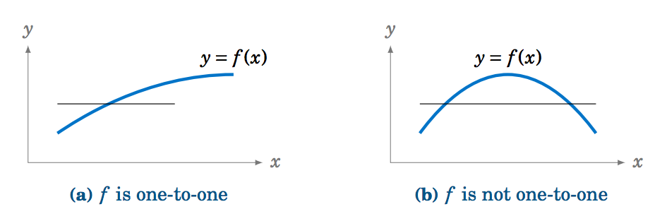
Figure 5.3.3 Horizontal rule for one-to-one functions

If a function $f $ is one-to-one on its domain, then $f $ has an inverse function, denoted by $f^{-1} $, such that $y=f(x) $ if and only if $f^{-1}(y) = x $. The domain of $f^{-1} $ is the range of $f $.

The basic idea is that $f^{-1} $ "undoes'' what $f $ does, and vice versa. In other words,
\[\nonumber \begin{alignat*}{3}
f^{-1}(f(x)) ~&=~ x \quad&&\text{for all $x $ in the domain of $f $, and}\\ \nonumber
f(f^{-1}(y)) ~&=~ y \quad&&\text{for all $y $ in the range of $f $.}
\end{alignat*}\]

Theorem $\PageIndex{1}$

If $f$ is continuous and one to one, then \(f^{-1}\ is continuous on its domain.

Inverse Trigonometric functions

We know from their graphs that none of the trigonometric functions are one-to-one over their entire domains. However, we can restrict those functions to subsets of their domains where they are one-to-one. For example, $y=\sin\;x $ is one-to-one over the interval $\left[ -\frac{\pi}{2},\frac{\pi}{2} \right] $, as we see in the graph below:

$alt$

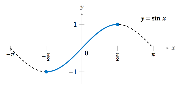
For $-\frac{\pi}{2} \le x \le \frac{\pi}{2} $ we have $-1 \le \sin\;x \le 1 $, so we can define the inverse sine function $y=\sin^{-1} x $ (sometimes called the arc sine and denoted by $y=\arcsin\;(x$) whose domain is the interval $[-1,1] $ and whose range is the interval $\left[ -\frac{\pi}{2},\frac{\pi}{2} \right] $. In other words:

\[ \begin{alignat}{3}
\sin^{-1} (\sin\;y) ~&=~ y \quad&&\text{for $-\tfrac{\pi}{2} \le y \le
\tfrac{\pi}{2}$}\label{eqn:arcsin1}\\
\sin\;(\sin^{-1} x) ~&=~ x \quad&&\text{for $-1 \le x \le 1$}\label{eqn:arcsin2}
\end{alignat}\]

Summary of Inverse Trigonometric functions

Lets illustrate the summary of Trigonometric functions and Inverse Trigonometric functions in following table:

Trigonometric function	graph of the Trigonometric function	Restricted domain and the range	Inverse Trigonometric function	graph of the Inverse Trigonometric function	Properties
$f(x)=\sin(x)$	$alt$	$\left[ -\frac{\pi}{2},\frac{\pi}{2} \right] $ and $[-1,1]$	$f^{-1}(x)=\sin^{-1} x 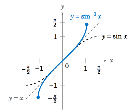$	$alt$
$f(x)=\cos(x)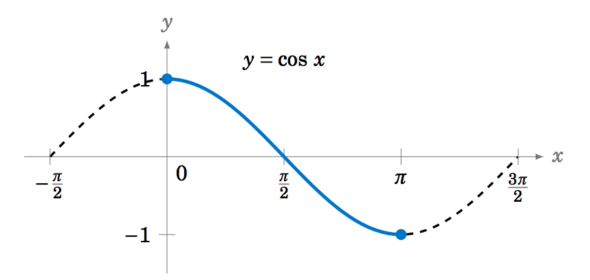$	$alt$	$[0,\pi]$ and $[-1,1]$	$f^{-1}(x)=\cos^{-1} x 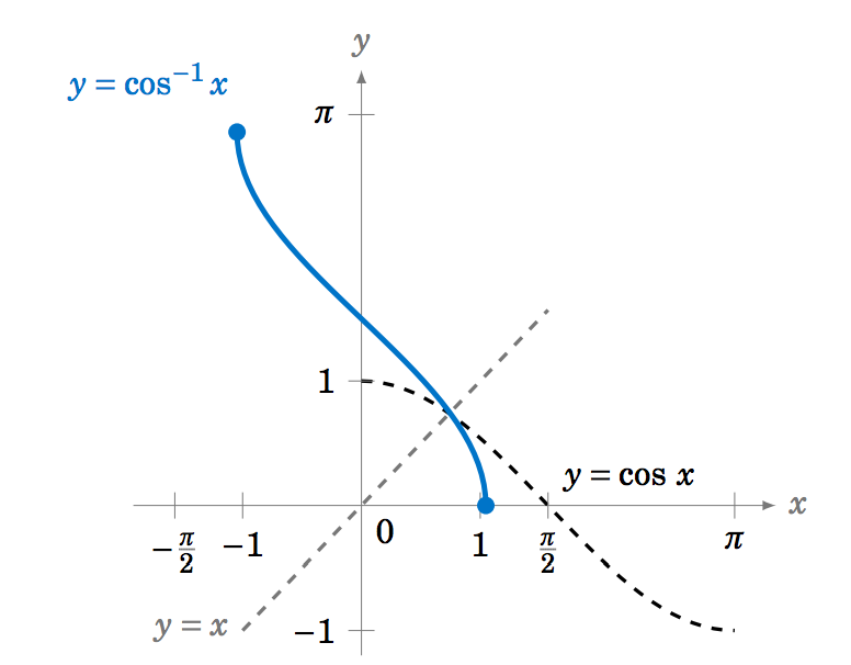$	$alt$	\[\begin{alignat}{3} \cos^{-1} (\cos\;y) ~&=~ y \quad&&\text{for $0 \le y \le \pi$}\label{eqn:arccos1}\\ \cos\;(\cos^{-1} x) ~&=~ x \quad&&\text{for $-1 \le x \le 1$}\label{eqn:arccos2} \end{alignat}\]
$f(x)=\tan(x)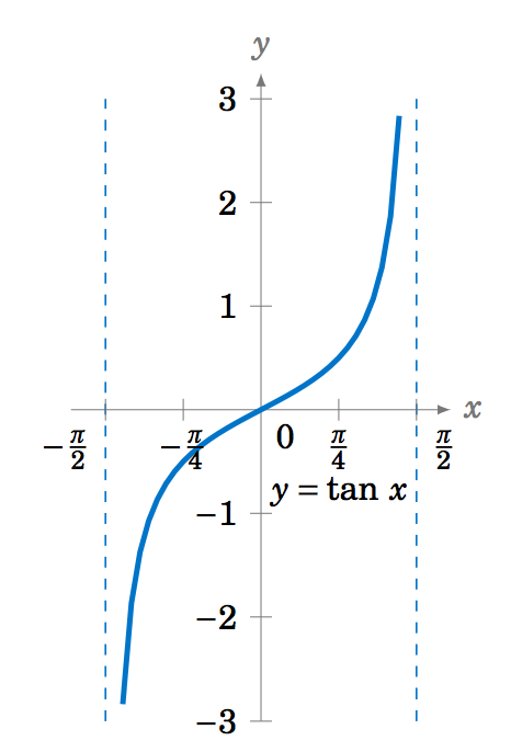$	$alt$	$\left( -\frac{\pi}{2},\frac{\pi}{2} \right) $ and $\mathbb{R}$	$f^{-1}(x)=\tan^{-1} x 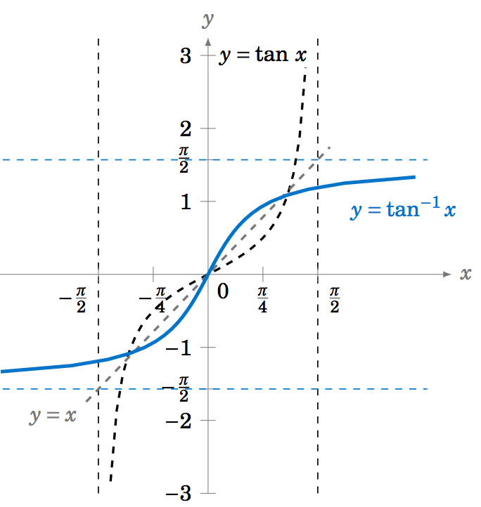$	$alt$	\[\begin{alignat}{3} \tan^{-1} (\tan\;y) ~&=~ y \quad&&\text{for $-\tfrac{\pi}{2} < y < \tfrac{\pi}{2}$}\label{eqn:arctan1}\\ \tan\;(\tan^{-1} x) ~&=~ x \quad&&\text{for all real $x$}\label{eqn:arctan2} \end{alignat}\]
$f(x)=\cot(x)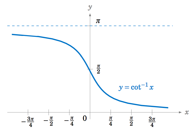$				$alt$	\[\begin{alignat}{3} \cot^{-1} (\cot\;y) ~&=~ y \quad&&\text{for $0 < y < \pi$}\label{eqn:arccot1}\\ \cot\;(\cot^{-1} x) ~&=~ x \quad&&\text{for all real $x$}\label{eqn:arccot2} \end{alignat}\]
$f(x)=\sec(x)$		$[0,\pi]$, with $x\ne \frac{\pi}{2}$ and $\mathbb{R}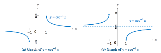$		$alt$	\[\begin{alignat}{3} \csc^{-1} (\csc\;y) ~&=~ y \quad&&\text{for $-\frac{\pi}{2} \le y \le \frac{\pi}{2} $, $y \ne 0$}\label{eqn:arccsc1}\\ \csc\;(\csc^{-1} x) ~&=~ x \quad&&\text{for $\|x\| \ge 1$}\label{eqn:arccsc2} \end{alignat}\] \[\begin{alignat}{3} \sec^{-1} (\sec\;y) ~&=~ y \quad&&\text{for $0 \le y \le \pi $, $y \ne \frac{\pi}{2}$}\label{eqn:arcsec1}\\ \sec\;(\sec^{-1} x) ~&=~ x \quad&&\text{for $\|x\| \ge 1$}\label{eqn:arcsec2} \end{alignat}\]

Below are examples:

Example $\PageIndex{1}$:

Find $\sin^{-1} \left(\sin\;\frac{\pi}{4}\right) $.

Solution

Since $-\frac{\pi}{2} \le \frac{\pi}{4} \le \frac{\pi}{2} $, we know that $\sin^{-1} \left(\sin\;\frac{\pi}{4}\right) = \boxed{\frac{\pi}{4}}\; $, by Equation \ref{eqn:arcsin1}.

Example $\PageIndex{2}$:

Find $\sin^{-1} \left(\sin\;\frac{5\pi}{4}\right) $.

Solution

Since $\frac{5\pi}{4} > \frac{\pi}{2} $, we can not use Equation \ref{eqn:arcsin1}. But we know that $\sin\;\frac{5\pi}{4} = -\frac{1}{\sqrt{2}} $. Thus, $\sin^{-1} \left(\sin\;\frac{5\pi}{4}\right) = \sin^{-1} \left( -\frac{1}{\sqrt{2}} \right) $ is, by definition, the angle $y $ such that $-\frac{\pi}{2} \le y \le \frac{\pi}{2} $ and $\sin\;y = -\frac{1}{\sqrt{2}} $. That angle is $y=-\frac{\pi}{4} $, since

\[\sin\;\left( -\tfrac{\pi}{4} \right) ~=~ -\sin\;\left( \tfrac{\pi}{4} \right) ~=~
-\tfrac{1}{\sqrt{2}} ~. \nonumber \]

Example $\PageIndex{3}$:

Find $\cos^{-1} \left(\cos\;\frac{\pi}{3}\right) $.

Solution

Since $0 \le \frac{\pi}{3} \le \pi $, we know that $\cos^{-1} \left(\cos\;\frac{\pi}{3}\right) = \boxed{\frac{\pi}{3}}\; $, by Equation \ref{eqn:arccos1}.

Example $\PageIndex{4}$:

Find $\cos^{-1} \left(\cos\;\frac{4\pi}{3}\right) $.

Solution

Since $\frac{4\pi}{3} > \pi $, we can not use Equation \ref{eqn:arccos1}. But we know that $\cos\;\frac{4\pi}{3} = -\frac{1}{2} $. Thus, $\cos^{-1} \left(\cos\;\frac{4\pi}{3}\right) = \cos^{-1} \left( -\frac{1}{2} \right) $ is, by definition, the angle $y $ such that $0 \le y \le \pi $ and $\cos\;y = -\frac{1}{2} $. That angle is $y=\frac{2\pi}{3} $ (i.e. $120^\circ$). Thus, $\cos^{-1} \left(\cos\;\frac{4\pi}{3}\right) = \boxed{\tfrac{2\pi}{3}}\; $.

Example $\PageIndex{5}$:

Find $\tan^{-1} \left(\tan\;\frac{\pi}{4}\right) $.

Solution

Since $-\tfrac{\pi}{2} \le \tfrac{\pi}{4} \le \tfrac{\pi}{2} $, we know that $\tan^{-1} \left(\tan\;\frac{\pi}{4}\right) = \boxed{\frac{\pi}{4}}\; $, by Equation \ref{eqn:arctan1}.

Example $\PageIndex{6}$:

Find $\tan^{-1} \left(\tan\;\pi\right) $.

Solution

Since $\pi > \tfrac{\pi}{2} $, we can not use Equation \ref{eqn:arctan1}. But we know that $\tan\;\pi = 0 $. Thus, $\tan^{-1} \left(\tan\;\pi\right) = \tan^{-1} 0 $ is, by definition, the angle $y $ such that $-\tfrac{\pi}{2} \le y \le \tfrac{\pi}{2} $ and $\tan\;y = 0 $. That angle is $y=0 $. Thus, $\tan^{-1} \left(\tan\;\pi \right) = \boxed{0}\; $.

Example$\PageIndex{7}$:

Find the exact value of $\cos\;\left(\sin^{-1}\;\left(-\frac{1}{4}\right)\right) $.

Solution

Let $\theta = \sin^{-1}\;\left(-\frac{1}{4}\right) $. We know that $-\tfrac{\pi}{2} \le \theta \le \tfrac{\pi}{2} $, so since $\sin\;\theta = -\frac{1}{4} < 0 $, $\theta $ must be in QIV. Hence $\cos\;\theta > 0 $. Thus,

\[ \cos^2 \;\theta ~=~ 1 ~-~ \sin^2 \;\theta ~=~ 1 ~-~ \left( -\frac{1}{4} \right)^2 ~=~\frac{15}{16}
\quad\Rightarrow\quad \cos\;\theta ~=~ \frac{\sqrt{15}}{4} ~. \nonumber \]

Note that we took the positive square root above since $\cos\;\theta > 0 $. Thus, $\cos\;\left(\sin^{-1}\;\left(-\frac{1}{4}\right)\right) = \boxed{\frac{\sqrt{15}}{4}}\; $.

Example $\PageIndex{8}$:

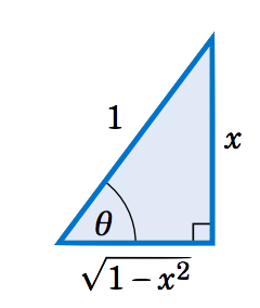
Show that $\tan\;(\sin^{-1} x) = \dfrac{x}{\sqrt{1 - x^2}} $ for $-1 < x < 1 $.

Solution

When $x=0 $, the Equation holds trivially, since

\[\nonumber \tan\;(\sin^{-1} 0) ~=~ \tan\;0 ~=~ 0 ~=~ \dfrac{0}{\sqrt{1 - 0^2}} ~.\]

Now suppose that $0 < x < 1 $. Let $\theta = \sin^{-1} x $. Then $\theta $ is in QI and $\sin\;\theta = x $. Draw a right triangle with an angle $\theta $ such that the opposite leg has length $x $ and the hypotenuse has length $1 $, as in Figure 5.3.10 (note that this is possible since $0 < x < 1$). Then $\sin\;\theta = \frac{x}{1} = x $. By the Pythagorean Theorem, the adjacent leg has length $\sqrt{1 - x^2} $. Thus, $\tan\;\theta = \frac{x}{\sqrt{1 - x^2}} $.

If $-1 < x < 0 $ then $\theta = \sin^{-1} x $ is in QIV. So we can draw the same triangle except that it would be "upside down'' and we would again have $\tan\;\theta = \frac{x}{\sqrt{1 - x^2}} $, since the tangent and sine have the same sign (negative) in QIV. Thus, $\tan\;(\sin^{-1} x) = \dfrac{x}{\sqrt{1 - x^2}} $ for $-1 < x < 1 $.

$alt$

Example $\PageIndex{9}$:

Prove the identity $\tan^{-1} x \;+\; \cot^{-1} x ~=~ \frac{\pi}{2} $.

Solution:

Let $\theta = \cot^{-1} x $. Using relations, we have

\[\nonumber \tan\;\left( \tfrac{\pi}{2} - \theta \right) ~=~ -\tan\;\left( \theta - \tfrac{\pi}{2} \right)
~=~ \cot\;\theta ~=~ \cot\;(\cot^{-1} x) ~=~ x ~,\]

by Equation \ref{eqn:arccot2}. So since $\tan\;(\tan^{-1} x) = x $ for all $x $, this means that $\tan\;(\tan^{-1} x) = \tan\;\left( \tfrac{\pi}{2} - \theta \right) $. Thus, $\tan\;(\tan^{-1} x) = \tan\;\left( \tfrac{\pi}{2} - \cot^{-1} x \right) $. Now, we know that $0 < \cot^{-1} x < \pi $, so $-\tfrac{\pi}{2} < \tfrac{\pi}{2} - \cot^{-1} x < \tfrac{\pi}{2} $, i.e. $\tfrac{\pi}{2} - \cot^{-1} x $ is in the restricted subset on which the tangent function is one-to-one. Hence, $\tan\;(\tan^{-1} x) = \tan\;\left( \tfrac{\pi}{2} - \cot^{-1} x \right)$ implies that $\tan^{-1} x = \tfrac{\pi}{2} - \cot^{-1} x $, which proves the identity.

Continuity of Inverse Trigonometric functions

Example $\PageIndex{1}$:

Let $f(x)= \frac{3 \sec^{-1} (x)}{4-\tan^{-1}( x)}$. Find the values(if any) for which $f(x)$ is continuous.

Exercise $\PageIndex{1}$

Let $f(x)= \frac{3 \sec^{-1} (x)}{8+2\tan^{-1}( x)}$. Find the values(if any) for which $f(x)$ is continuous.

Answer

Limit of Inverse Trigonometric functions

Theorem $\PageIndex{1}$

$lim_{x \rightarrow \infty} \tan^{-1}( x) = \frac{\pi}{2} $.

$lim_{x \rightarrow -\infty} \tan^{-1}( x) = -\frac{\pi}{2} $.

$lim_{x \rightarrow \infty} \sec^{-1} (x)=\lim _{x \rightarrow \infty} \sec^{-1} (x )= \frac{\pi}{2} $.

Example $\PageIndex{1}$:

Find $\lim_{x \rightarrow \infty} sin\left( 2\tan^{-1}( x)\right)$.

Exercise $\PageIndex{1}$

Find $\lim_{x \rightarrow -\infty} sin\left( 2\tan^{-1}( x)\right)$.

Answer

Contributors and Attributions

Michael Corral (Schoolcraft College). The content of this page is distributed under the terms of the GNU Free Documentation License, Version 1.2.
Gilbert Strang (MIT) and Edwin “Jed” Herman (Harvey Mudd) with many contributing authors. This content by OpenStax is licensed with a CC-BY-SA-NC 4.0 license. Download for free at http://cnx.org.
Pamini Thangarajah (Mount Royal University, Calgary, Alberta, Canada)

Trigonometric function	graph of the Trigonometric function	Restricted domain and the range	Inverse Trigonometric function	graph of the Inverse Trigonometric function	Properties
\(f(x)=\sin(x)\)	$alt$	\(\left[ -\frac{\pi}{2},\frac{\pi}{2} \right] \) and \([-1,1]\)	\(f^{-1}(x)=\sin^{-1} x \)	$alt$
\(f(x)=\cos(x)\)	$alt$	\([0,\pi]\) and \([-1,1]\)	\(f^{-1}(x)=\cos^{-1} x \)	$alt$	\[\begin{alignat}{3} \cos^{-1} (\cos\;y) ~&=~ y \quad&&\text{for \(0 \le y \le \pi\)}\label{eqn:arccos1}\\ \cos\;(\cos^{-1} x) ~&=~ x \quad&&\text{for \(-1 \le x \le 1\)}\label{eqn:arccos2} \end{alignat}\]
\(f(x)=\tan(x)\)	$alt$	\(\left( -\frac{\pi}{2},\frac{\pi}{2} \right) \) and \(\mathbb{R}\)	\(f^{-1}(x)=\tan^{-1} x \)	$alt$	\[\begin{alignat}{3} \tan^{-1} (\tan\;y) ~&=~ y \quad&&\text{for \(-\tfrac{\pi}{2} < y < \tfrac{\pi}{2}\)}\label{eqn:arctan1}\\ \tan\;(\tan^{-1} x) ~&=~ x \quad&&\text{for all real \(x\)}\label{eqn:arctan2} \end{alignat}\]
\(f(x)=\cot(x)\)				$alt$	\[\begin{alignat}{3} \cot^{-1} (\cot\;y) ~&=~ y \quad&&\text{for \(0 < y < \pi\)}\label{eqn:arccot1}\\ \cot\;(\cot^{-1} x) ~&=~ x \quad&&\text{for all real \(x\)}\label{eqn:arccot2} \end{alignat}\]
\(f(x)=\sec(x)\)		\([0,\pi]\), with \(x\ne \frac{\pi}{2}\) and \(\mathbb{R}\)		$alt$	\[\begin{alignat}{3} \csc^{-1} (\csc\;y) ~&=~ y \quad&&\text{for \(-\frac{\pi}{2} \le y \le \frac{\pi}{2} \), \(y \ne 0\)}\label{eqn:arccsc1}\\ \csc\;(\csc^{-1} x) ~&=~ x \quad&&\text{for \(\|x\| \ge 1\)}\label{eqn:arccsc2} \end{alignat}\] \[\begin{alignat}{3} \sec^{-1} (\sec\;y) ~&=~ y \quad&&\text{for \(0 \le y \le \pi \), \(y \ne \frac{\pi}{2}\)}\label{eqn:arcsec1}\\ \sec\;(\sec^{-1} x) ~&=~ x \quad&&\text{for \(\|x\| \ge 1\)}\label{eqn:arcsec2} \end{alignat}\]

Search

Text Color

Text Size

Margin Size

Font Type