
6.1: Parametric equations - Tangent lines and arc length


- Last updated
- Dec 21, 2020
- Save as PDF
This page is a draft and is under active development.

( \newcommand{\kernel}{\mathrm{null}\,}\)
In this section we examine parametric equations and their graphs. In the two-dimensional coordinate system, parametric equations are useful for describing curves that are not necessarily functions. The parameter is an independent variable that both
Parametric Equations and Their Graphs
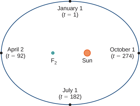
Consider the orbit of Earth around the Sun. Our year lasts approximately 365.25 days, but for this discussion we will use 365 days. On January 1 of each year, the physical location of Earth with respect to the Sun is nearly the same, except for leap years, when the lag introduced by the extra
The number of the day in a year can be considered a variable that determines Earth’s position in its orbit. As Earth revolves around the Sun, its physical location changes relative to the Sun. After one full year, we are back where we started, and a new year begins. According to Kepler’s laws of planetary motion, the shape of the orbit is elliptical, with the Sun at one focus of the ellipse. We study this idea in more detail in Conic Sections.
Figure
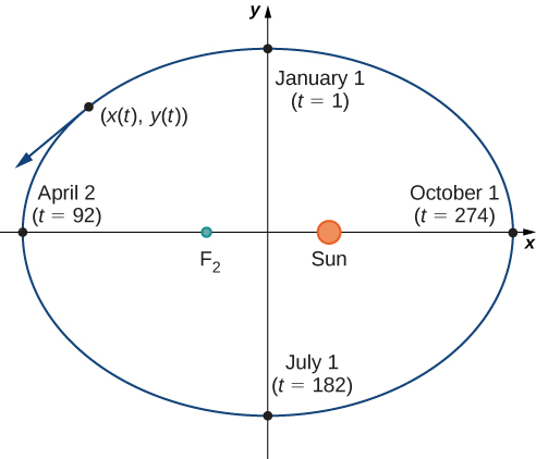
We can determine the functions for
A curve in the
Definition: Parametric Equations
If
and
are called parametric equations and
Notice in this definition that x and y are used in two ways. The first is as functions of the independent variable
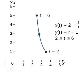
Example
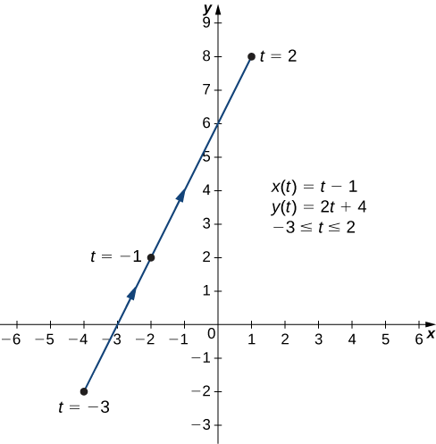
Sketch the curves described by the following parametric equations:
Solution
a. To create a graph of this curve, first set up a table of values. Since the independent variable in both
| −3 | −4 | −2 |
| −2 | −3 | 0 |
| −1 | −2 | 2 |
| 0 | −1 | 4 |
| 1 | 0 | 6 |
| 2 | 1 | 8 |
The second and third columns in this table provide a set of points to be plotted. The graph of these points appears in Figure
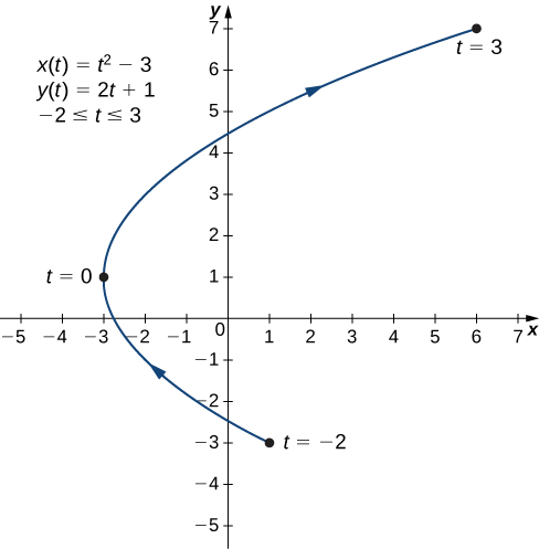
b. To create a graph of this curve, again set up a table of values.
| −2 | 1 | −3 |
| −1 | −2 | −1 |
| 0 | −3 | 1 |
| 1 | −2 | 3 |
| 2 | 1 | 5 |
| 3 | 6 | 7 |
The second and third columns in this table give a set of points to be plotted (Figure
c. In this case, use multiples of
| 0 | 4 | 0 | −23√≈−3.5 | 2 | |
| 2 | −2 | ||||
| 2 | 0 | −4 | |||
| 0 | 4 | 2 | |||
| −2 | 2 | ||||
| 2 | 4 | 0 | |||
| −4 | 0 |
The graph of this plane curve appears in the following graph.
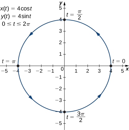
This is the graph of a circle with radius 4 centered at the origin, with a counterclockwise orientation. The starting point and ending points of the curve both have coordinates
Exercise
Sketch the curve described by the parametric equations
- Hint
-
Make a table of values for
- Answer
-
Eliminating the Parameter
To better understand the graph of a curve represented parametrically, it is useful to rewrite the two equations as a single equation relating the variables
over the region
Solving Equation
This can be substituted into Equation
Equation
Example
Eliminate the parameter for each of the plane curves described by the following parametric equations and describe the resulting graph.
Solution
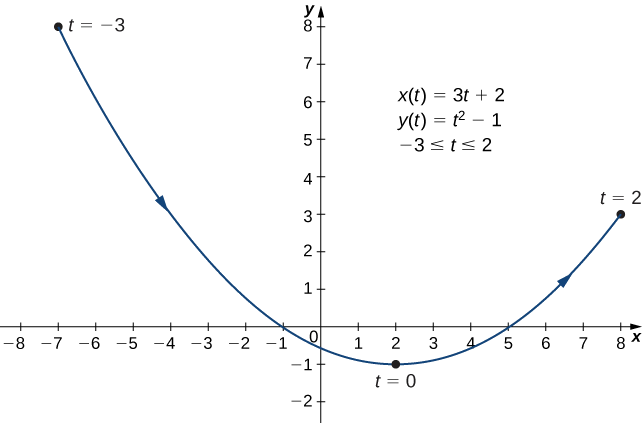
a. To eliminate the parameter, we can solve either of the equations for
Note that when we square both sides it is important to observe that
This is the equation of a parabola opening upward. There is, however, a domain restriction because of the limits on the parameter
b. Sometimes it is necessary to be a bit creative in eliminating the parameter. The parametric equations for this example are
and
Solving either equation for t directly is not advisable because sine and cosine are not one-to-one functions. However, dividing the first equation by 4 and the second equation by 3 (and suppressing the t) gives us
and
Now use the Pythagorean identity
This is the equation of a horizontal ellipse centered at the origin, with semi-major axis 4 and semi-minor axis 3 as shown in the following graph.
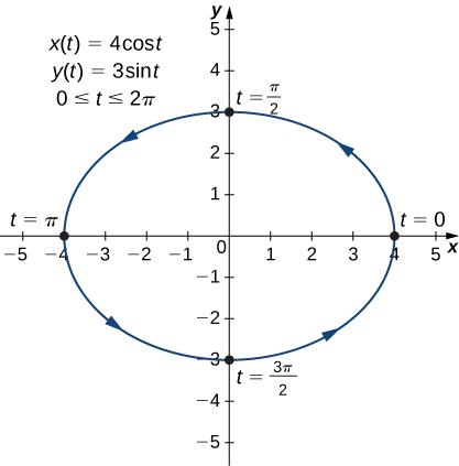
As t progresses from
Exercise
Eliminate the parameter for the plane curve defined by the following parametric equations and describe the resulting graph.
- Hint
-
Solve one of the equations for t and substitute into the other equation.
- Answer
-
So far we have seen the method of eliminating the parameter, assuming we know a set of parametric equations that describe a plane curve. What if we would like to start with the equation of a curve and determine a pair of parametric equations for that curve? This is certainly possible, and in fact it is possible to do so in many different ways for a given curve. The process is known as parameterization of a curve.
Example
Find two different pairs of parametric equations to represent the graph of
Solution
First, it is always possible to parameterize a curve by defining
Since there is no restriction on the domain in the original graph, there is no restriction on the values of
We have complete freedom in the choice for the second parameterization. For example, we can choose
Therefore, a second parameterization of the curve can be written as
Exercise
Find two different sets of parametric equations to represent the graph of
- Hint
-
Follow the steps in Example. Remember we have freedom in choosing the parameterization for
- Answer
-
One possibility is
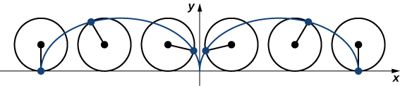
Cycloids and Other Parametric Curves
Imagine going on a bicycle ride through the country. The tires stay in contact with the road and rotate in a predictable pattern. Now suppose a very determined ant is tired after a long day and wants to get home. So he hangs onto the side of the tire and gets a free ride. The path that this ant travels down a straight road is called a cycloid (Figure
To see why this is true, consider the path that the center of the wheel takes. The center moves along the x-axis at a constant height equal to the radius of the wheel. If the radius is a, then the coordinates of the center can be given by the equations
for any value of
(The negative sign is needed to reverse the orientation of the curve. If the negative sign were not there, we would have to imagine the wheel rotating counterclockwise.) Adding these equations together gives the equations for the cycloid.
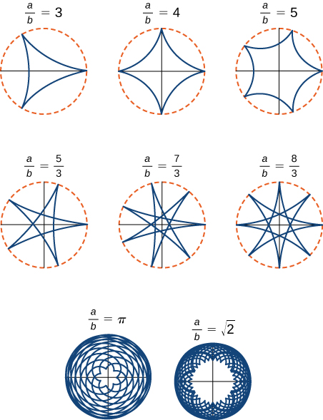
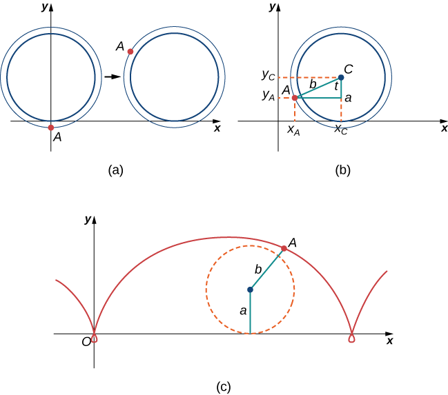
Now suppose that the bicycle wheel doesn’t travel along a straight road but instead moves along the inside of a larger wheel, as in Figure
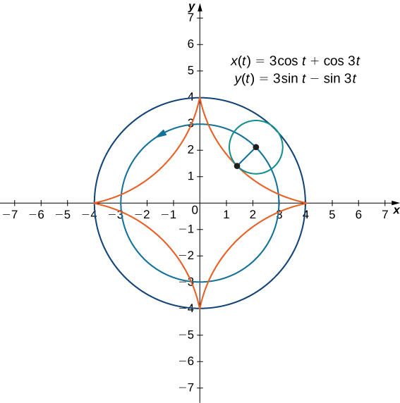
The general parametric equations for a hypocycloid are
These equations are a bit more complicated, but the derivation is somewhat similar to the equations for the cycloid. In this case we assume the radius of the larger circle is a and the radius of the smaller circle is b. Then the center of the wheel travels along a circle of radius
The ratio
The Witch of Agnesi
Many plane curves in mathematics are named after the people who first investigated them, like the folium of Descartes or the spiral of Archimedes. However, perhaps the strangest name for a curve is the witch of Agnesi. Why a witch?
Maria Gaetana Agnesi (1718–1799) was one of the few recognized women mathematicians of eighteenth-century Italy. She wrote a popular book on analytic geometry, published in 1748, which included an interesting curve that had been studied by Fermat in 1630. The mathematician Guido Grandi showed in 1703 how to construct this curve, which he later called the “versoria,” a Latin term for a rope used in sailing. Agnesi used the Italian term for this rope, “versiera,” but in Latin, this same word means a “female goblin.” When Agnesi’s book was translated into English in 1801, the translator used the term “witch” for the curve, instead of rope. The name “witch of Agnesi” has stuck ever since.
The witch of Agnesi is a curve defined as follows: Start with a circle of radius a so that the points
Witch of Agnesi curves have applications in physics, including modeling water waves and distributions of spectral lines. In probability theory, the curve describes the probability density function of the Cauchy distribution. In this project you will parameterize these curves.
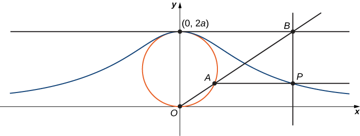
1. On the figure, label the following points, lengths, and angle:
a. C is the point on the x-axis with the same x-coordinate as A.
b. x is the x-coordinate of P, and y is the y-coordinate of P.
c. E is the point
d. F is the point on the line segment OA such that the line segment EF is perpendicular to the line segment OA.
e. b is the distance from O to F.
f. c is the distance from F to A.
g. d is the distance from O to B.
h.
The goal of this project is to parameterize the witch using
2. Show that
3. Note that
4. In terms of
5. Show that
6. Show that
7. Show that
8. Conclude that a parameterization of the given witch curve is
9. Use your parameterization to show that the given witch curve is the graph of the function
Travels with My Ant: The Curtate and Prolate Cycloids
Earlier in this section, we looked at the parametric equations for a cycloid, which is the path a point on the edge of a wheel traces as the wheel rolls along a straight path. In this project we look at two different variations of the cycloid, called the curtate and prolate cycloids.
First, let’s revisit the derivation of the parametric equations for a cycloid. Recall that we considered a tenacious ant trying to get home by hanging onto the edge of a bicycle tire. We have assumed the ant climbed onto the tire at the very edge, where the tire touches the ground. As the wheel rolls, the ant moves with the edge of the tire (Figure).
As we have discussed, we have a lot of flexibility when parameterizing a curve. In this case we let our parameter t represent the angle the tire has rotated through. Looking at Figure
Furthermore, letting
Then
Note that these are the same parametric representations we had before, but we have now assigned a physical meaning to the parametric variable
After a while the ant is getting dizzy from going round and round on the edge of the tire. So he climbs up one of the spokes toward the center of the wheel. By climbing toward the center of the wheel, the ant has changed his path of motion. The new path has less up-and-down motion and is called a curtate cycloid (Figure
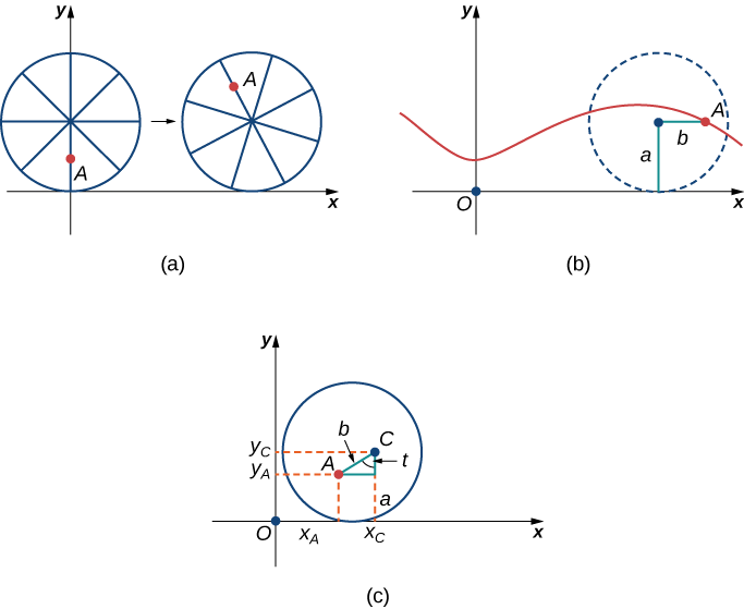
1. What is the position of the center of the wheel after the tire has rotated through an angle of
2. Use geometry to find expressions for
3. On the basis of your answers to parts 1 and 2, what are the parametric equations representing the curtate cycloid?
Once the ant’s head clears, he realizes that the bicyclist has made a turn, and is now traveling away from his home. So he drops off the bicycle tire and looks around. Fortunately, there is a set of train tracks nearby, headed back in the right direction. So the ant heads over to the train tracks to wait. After a while, a train goes by, heading in the right direction, and he manages to jump up and just catch the edge of the train wheel (without getting squished!).
The ant is still worried about getting dizzy, but the train wheel is slippery and has no spokes to climb, so he decides to just hang on to the edge of the wheel and hope for the best. Now, train wheels have a flange to keep the wheel running on the tracks. So, in this case, since the ant is hanging on to the very edge of the flange, the distance from the center of the wheel to the ant is actually greater than the radius of the wheel (Figure).
The setup here is essentially the same as when the ant climbed up the spoke on the bicycle wheel. We let b denote the distance from the center of the wheel to the ant, and we let t represent the angle the tire has rotated through. Additionally, we let
When the distance from the center of the wheel to the ant is greater than the radius of the wheel, his path of motion is called a prolate cycloid. A graph of a prolate cycloid is shown in the figure.
4. Using the same approach you used in parts 1– 3, find the parametric equations for the path of motion of the ant.
5. What do you notice about your answer to part 3 and your answer to part 4?
Notice that the ant is actually traveling backward at times (the “loops” in the graph), even though the train continues to move forward. He is probably going to be really dizzy by the time he gets home!
Key Concepts
- Parametric equations provide a convenient way to describe a curve. A parameter can represent time or some other meaningful quantity.
- It is often possible to eliminate the parameter in a parameterized curve to obtain a function or relation describing that curve.
- There is always more than one way to parameterize a curve.
- Parametric equations can describe complicated curves that are difficult or perhaps impossible to describe using rectangular coordinates.
Glossary
- cycloid
- the curve traced by a point on the rim of a circular wheel as the wheel rolls along a straight line without slippage
- cusp
- a pointed end or part where two curves meet
- orientation
- the direction that a point moves on a graph as the parameter increases
- parameter
- an independent variable that both x and y depend on in a parametric curve; usually represented by the variable t
- parametric curve
- the graph of the parametric equations
- parametric equations
- the equations
- parameterization of a curve
- rewriting the equation of a curve defined by a function
Contributors and Attributions
Gilbert Strang (MIT) and Edwin “Jed” Herman (Harvey Mudd) with many contributing authors. This content by OpenStax is licensed with a CC-BY-SA-NC 4.0 license. Download for free at http://cnx.org.