1.4E: Exercises

Exercise \(\PageIndex{1}\)

In the following exercises, use appropriate substitutions to write down the Maclaurin series for the given binomial.

1. \(\displaystyle (1−x)^{1/3}\)

2. \(\displaystyle (1+x^2)^{−1/3}\)

Answer

\(\displaystyle (1+x^2)^{−1/3}=\sum_{n=0}^∞(^{−\frac{1}{3}}_n)x^{2n}\)

3. \(\displaystyle (1−x)^{1.01}\)

4. \(\displaystyle (1−2x)^{2/3}\)

Answer

\(\displaystyle (1−2x)^{2/3}=\sum_{n=0}^∞(−1)^n2^n(^{\frac{2}{3}}_n)x^n\)

Exercise \(\PageIndex{2}\)

In the following exercises, use the substitution \(\displaystyle (b+x)^r=(b+a)^r(1+\frac{x−a}{b+a})^r\) in the binomial expansion to find the Taylor series of each function with the given center.

1. \(\sqrt{x+2}\) at \(\displaystyle a=0\)

2. \(\displaystyle \sqrt{x^2+2}\) at \(\displaystyle a=0\)

Answer

\(\displaystyle \sqrt{2+x^2}=\sum_{n=0}^∞2^{(1/2)−n}(^{\frac{1}{2}}_n)x^{2n};(∣x^2∣<2)\)

3. \(\displaystyle \sqrt{x+2}\) at \(\displaystyle a=1\)

4. \(\displaystyle \sqrt{2x−x^2}\) at \(\displaystyle a=1\) (Hint: \(\displaystyle 2x−x^2=1−(x−1)^2\))

Answer

\(\displaystyle \sqrt{2x−x^2}=\sqrt{1−(x−1)^2}\) so \(\displaystyle \sqrt{2x−x^2}=\sum_{n=0}^∞(−1)^n(^{\frac{1}{2}}_n)(x−1)^{2n}\)

5. \(\displaystyle (x−8)^{1/3}\) at \(\displaystyle a=9\)

6. \(\displaystyle \sqrt{x}\) at \(\displaystyle a=4\)

Answer

\(\displaystyle \sqrt{x}=2\sqrt{1+\frac{x−4}{4}}\) so \(\displaystyle \sqrt{x}=\sum_{n=0}^∞2^{1−2n}(^{\frac{1}{2}}_n)(x−4)^n\)

7. \(\displaystyle x^{1/3}\) at \(\displaystyle a=27\)

8. \(\displaystyle \sqrt{x}\) at \(\displaystyle x=9\)

Answer

\(\displaystyle \sqrt{x}=\sum_{n=0}^∞3^{1−3n}(^{\frac{1}{2}}_n)(x−9)^n\)

Exercise \(\PageIndex{3}\)

In the following exercises, use the binomial theorem to estimate each number, computing enough terms to obtain an estimate accurate to an error of at most \(\displaystyle 1/1000.\)

1. \(\displaystyle (15)^{1/4}\) using \(\displaystyle (16−x)^{1/4}\)

2. \(\displaystyle (1001)^{1/3}\) using \(\displaystyle (1000+x)^{1/3}\)

Answer

\(\displaystyle 10(1+\frac{x}{1000})^{1/3}=\sum_{n=0}^∞10^{1−3n}(^{\frac{1}{3}}_n)x^n\). Using, for example, a fourth-degree estimate at \(\displaystyle x=1\) gives \(\displaystyle (1001)^{1/3}≈10(1+(^{\frac{1}{3}}_1)10^{−3}+(^{\frac{1}{3}}_2)10^{−6}+(^{\frac{1}{3}}_3)10^{−9}+(^{\frac{1}{3}}_4)10^{−12})=10(1+\frac{1}{3.10^3}−\frac{1}{9.10^6}+\frac{5}{81.10^9}−\frac{10}{243.10^{12}})=10.00333222...\) whereas \(\displaystyle (1001)^{1/3}=10.00332222839093....\) Two terms would suffice for three-digit accuracy.

Exercise \(\PageIndex{4}\)

In the following exercises, use the binomial approximation \(\displaystyle \sqrt{1−x}≈1−\frac{x}{2}−\frac{x^2}{8}−\frac{x^3}{16}−\frac{5x^4}{128}−\frac{7x^5}{256}\) for \(\displaystyle |x|<1\) to approximate each number. Compare this value to the value given by a scientific calculator.

1. \(\displaystyle \frac{1}{\sqrt{2}}\) using \(\displaystyle x=\frac{1}{2}\) in \(\displaystyle (1−x)^{1/2}\)

2. \(\displaystyle \sqrt{5}=5×\frac{1}{\sqrt{5}}\) using \(\displaystyle x=\frac{4}{5}\) in \(\displaystyle (1−x)^{1/2}\)

Answer

The approximation is \(\displaystyle 2.3152\); the CAS value is \(\displaystyle 2.23….\)

3. \(\displaystyle \sqrt{3}=\frac{3}{\sqrt{3}}\) using \(\displaystyle x=\frac{2}{3}\) in \(\displaystyle (1−x)^{1/2}\)

4. \(\displaystyle \sqrt{6}\) using \(\displaystyle x=\frac{5}{6}\) in \(\displaystyle (1−x)^{1/2}\)

Answer

The approximation is \(\displaystyle 2.583…\); the CAS value is \(\displaystyle 2.449….\)

5. Integrate the binomial approximation of \(\displaystyle \sqrt{1−x}\) to find an approximation of \(\displaystyle ∫^x_0\sqrt{1−t}dt\).

6. Recall that the graph of \(\displaystyle \sqrt{1−x^2}\) is an upper semicircle of radius \(\displaystyle 1\). Integrate the binomial approximation of \(\displaystyle \sqrt{1−x^2}\) up to order \(\displaystyle 8\) from \(\displaystyle x=−1\) to \(\displaystyle x=1\) to estimate \(\displaystyle \frac{π}{2}\).

Answer

\(\displaystyle \sqrt{1−x^2}=1−\frac{x^2}{2}−\frac{x^4}{8}−\frac{x^6}{16}−\frac{5x^8}{128}+⋯.\) Thus \(\displaystyle ∫^1_{−1}\sqrt{1−x^2}dx=x−\frac{x^3}{6}−\frac{x^5}{40}−\frac{x^7}{7⋅16}−\frac{5x^9}{9⋅128}+⋯∣^1_{−1}≈2−\frac{1}{3}−\frac{1}{20}−\frac{1}{56}−\frac{10}{9⋅128}+error=1.590...\) whereas \(\displaystyle \frac{π}{2}=1.570...\)

Exercise \(\PageIndex{5}\)

In the following exercises, use the expansion \(\displaystyle (1+x)^{1/3}=1+\frac{1}{3}x−\frac{1}{9}x^2+\frac{5}{81}x^3−\frac{10}{243}x^4+⋯\) to write the first five terms (not necessarily a quartic polynomial) of each expression.

1. \(\displaystyle (1+4x)^{1/3};a=0\)

2. \(\displaystyle (1+4x)^{4/3};a=0\)

Answer

\(\displaystyle (1+x)^{4/3}=(1+x)(1+\frac{1}{3}x−\frac{1}{9}x^2+\frac{5}{81}x^3−\frac{10}{243}x^4+⋯)=1+\frac{4x}{3}+\frac{2x^2}{9}−\frac{4x^3}{81}+\frac{5x^4}{243}+⋯\)

3. \(\displaystyle (3+2x)^{1/3};a=−1\)

4. \(\displaystyle (x^2+6x+10)^{1/3};a=−3\)

Answer

\(\displaystyle (1+(x+3)^2)^{1/3}=1+\frac{1}{3}(x+3)^2−\frac{1}{9}(x+3)^4+\frac{5}{81}(x+3)^6−\frac{10}{243}(x+3)^8+⋯\)

5. Use \(\displaystyle (1+x)^{1/3}=1+\frac{1}{3}x−\frac{1}{9}x^2+\frac{5}{81}x^3−\frac{10}{243}x^4+⋯\) with \(\displaystyle x=1\) to approximate \(\displaystyle 2^{1/3}\).

6. Use the approximation \(\displaystyle (1−x)^{2/3}=1−\frac{2x}{3}−\frac{x^2}{9}−\frac{4x^3}{81}−\frac{7x^4}{243}−\frac{14x^5}{729}+⋯\) for \(\displaystyle |x|<1\) to approximate \(\displaystyle 2^{1/3}=2.2^{−2/3}\).

Answer

Twice the approximation is \(\displaystyle 1.260…\) whereas \(\displaystyle 2^{1/3}=1.2599....\)

7. Find the \(\displaystyle 25th\) derivative of \(\displaystyle f(x)=(1+x^2)^{13}\) at \(\displaystyle x=0\).

8. Find the \(\displaystyle 99\) th derivative of \(\displaystyle f(x)=(1+x^4)^{25}\).

Answer

\(\displaystyle f^{(99)}(0)=0\)

Exercise \(\PageIndex{6}\)

In the following exercises, find the Maclaurin series of each function.

1. \(\displaystyle f(x)=xe^{2x}\)

2. \(\displaystyle f(x)=2^x\)

Answer

\(\displaystyle \sum_{n=0}^∞\frac{(ln(2)x)^n}{n!}\)

3. \(\displaystyle f(x)=\frac{sinx}{x}\)

4. \(\displaystyle f(x)=\frac{sin(\sqrt{x})}{\sqrt{x}},(x>0),\)

Answer

For \(\displaystyle x>0,sin(\sqrt{x})=\sum_{n=0}^∞(−1)^n\frac{x^{(2n+1)/2}}{\sqrt{x}(2n+1)!}=\sum_{n=0}^∞(−1)^n\frac{x^n}{(2n+1)!}\).

5. \(\displaystyle f(x)=sin(x^2)\)

6. \(\displaystyle f(x)=e^{x^3}\)

Answer

\(\displaystyle e^{x^3}=\sum_{n=0}^∞\frac{x^{3n}}{n!}\)

7. \(\displaystyle f(x)=cos^2x\) using the identity \(\displaystyle cos^2x=\frac{1}{2}+\frac{1}{2}cos(2x)\)

8. \(\displaystyle f(x)=sin^2x\) using the identity \(\displaystyle sin^2x=\frac{1}{2}−\frac{1}{2}cos(2x)\)

Answer

\(\displaystyle sin^2x=−\sum_{k=1}^∞\frac{(−1)^k2^{2k−1}x^{2k}}{(2k)!}\)

Exercise \(\PageIndex{7}\)

In the following exercises, find the Maclaurin series of \(\displaystyle F(x)=∫^x_0f(t)dt\) by integrating the Maclaurin series of \(\displaystyle f\) term by term. If \(\displaystyle f\) is not strictly defined at zero, you may substitute the value of the Maclaurin series at zero.

1. \(\displaystyle F(x)=∫^x_0e^{−t^2}dt;f(t)=e^{−t^2}=\sum_{n=0}^∞(−1)^n\frac{t^{2n}}{n!}\)

2. \(\displaystyle F(x)=tan^{−1}x;f(t)=\frac{1}{1+t^2}=\sum_{n=0}^∞(−1)^nt^{2n}\)

Answer

\(\displaystyle tan^{−1}x=\sum_{k=0}^∞\frac{(−1)^kx^{2k+1}}{2k+1}\)

3. \(\displaystyle F(x)=tanh^{−1}x;f(t)=\frac{1}{1−t^2}=\sum_{n=0}^∞t^{2n}\)

4. \(\displaystyle F(x)=sin^{−1}x;f(t)=\frac{1}{\sqrt{1−t^2}}=\sum_{k=0}^∞(^{\frac{1}{2}}_k)\frac{t^{2k}}{k!}\)

Answer

\(\displaystyle sin^{−1}x=\sum_{n=0}^∞(^{\frac{1}{2}}_n)\frac{x^{2n+1}}{(2n+1)n!}\)

5. \(\displaystyle F(x)=∫^x_0\frac{sint}{t}dt;f(t)=\frac{sint}{t}=\sum_{n=0}^∞(−1)^n\frac{t^{2n}}{(2n+1)!}\)

6. \(\displaystyle F(x)=∫^x_0cos(\sqrt{t})dt;f(t)=\sum_{n=0}^∞(−1)^n\frac{x^n}{(2n)!}\)

Answer

\(\displaystyle F(x)=\sum_{n=0}^∞(−1)^n\frac{x^{n+1}}{(n+1)(2n)!}\)

7. \(\displaystyle F(x)=∫^x_0\frac{1−cost}{t^2}dt;f(t)=\frac{1−cost}{t^2}=\sum_{n=0}^∞(−1)^n\frac{t^{2n}}{(2n+2)!}\)

8. \(\displaystyle F(x)=∫^x_0\frac{ln(1+t)}{t}dt;f(t)=\sum_{n=0}^∞(−1)^n\frac{t^n}{n+1}\)

Answer

\(\displaystyle F(x)=\sum_{n=1}^∞(−1)^{n+1}\frac{x^n}{n^2}\)

Exercise \(\PageIndex{8}\)

In the following exercises, compute at least the first three nonzero terms (not necessarily a quadratic polynomial) of the Maclaurin series of \(\displaystyle f\).

1. \(\displaystyle f(x)=sin(x+\frac{π}{4})=sinxcos(\frac{π}{4})+cosxsin(\frac{π}{4})\)

2. \(\displaystyle f(x)=tanx\)

Answer

\(\displaystyle x+\frac{x^3}{3}+\frac{2x^5}{15}+⋯\)

3. \(\displaystyle f(x)=ln(cosx)\)

4. \(\displaystyle f(x)=e^xcosx\)

Answer

\(\displaystyle 1+x−\frac{x^3}{3}−\frac{x^4}{6}+⋯\)

5. \(\displaystyle f(x)=e^{sinx}\)

6. \(\displaystyle f(x)=sec^2x\)

Answer

\(\displaystyle 1+x^2+\frac{2x^4}{3}+\frac{17x^6}{45}+⋯\)

7. \(\displaystyle f(x)=tanhx\)

8. \(\displaystyle f(x)=\frac{tan\sqrt{x}}{\sqrt{x}}\) (see expansion for \(\displaystyle tanx\))

Answer

Using the expansion for \(\displaystyle tanx\) gives \(\displaystyle 1+\frac{x}{3}+\frac{2x^2}{15}\).

Exercise \(\PageIndex{9}\)

In the following exercises, find the radius of convergence of the Maclaurin series of each function.

1. \(\displaystyle ln(1+x)\)

2. \(\displaystyle \frac{1}{1+x^2}\)

Answer

\(\displaystyle \frac{1}{1+x^2}=\sum_{n=0}^∞(−1)^nx^{2n}\) so \(\displaystyle R=1\) by the ratio test.

3. \(\displaystyle tan^{−1}x\)

4. \(\displaystyle ln(1+x^2)\)

Answer

\(\displaystyle ln(1+x^2)=\sum_{n=1}^∞\frac{(−1)^{n−1}}{n}x^{2n}\) so \(\displaystyle R=1\) by the ratio test.

5. Find the Maclaurin series of \(\displaystyle sinhx=\frac{e^x−e^{−x}}{2}\).

6. Find the Maclaurin series of \(\displaystyle coshx=\frac{e^x+e^{−x}}{2}\).

Answer

Add series of \(\displaystyle e^x\) and \(\displaystyle e^{−x}\) term by term. Odd terms cancel and \(\displaystyle coshx=\sum_{n=0}^∞\frac{x^{2n}}{(2n)!}\).

Exercise \(\PageIndex{10}\)

1. Differentiate term by term the Maclaurin series of \(\displaystyle sinhx\) and compare the result with the Maclaurin series of \(\displaystyle coshx\).

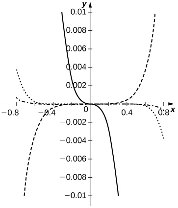
2. Let \(\displaystyle S_n(x)=\sum_{k=0}^n(−1)^k\frac{x^{2k+1}}{(2k+1)!}\) and \(\displaystyle C_n(x)=\sum_{n=0}^n(−1)^k\frac{x^{2k}}{(2k)!}\) denote the respective Maclaurin polynomials of degree \(\displaystyle 2n+1\) of \(\displaystyle sinx\) and degree \(\displaystyle 2n\) of \(\displaystyle cosx\). Plot the errors \(\displaystyle \frac{S_n(x)}{C_n(x)}−tanx\) for \(\displaystyle n=1,..,5\) and compare them to \(\displaystyle x+\frac{x^3}{3}+\frac{2x^5}{15}+\frac{17x^7}{315}−tanx\) on \(\displaystyle (−\frac{π}{4},\frac{π}{4})\).

Answer

The ratio \(\displaystyle \frac{S_n(x)}{C_n(x)}\) approximates \(\displaystyle tanx\) better than does \(\displaystyle p_7(x)=x+\frac{x^3}{3}+\frac{2x^5}{15}+\frac{17x^7}{315}\) for \(\displaystyle N≥3\). The dashed curves are \(\displaystyle \frac{S_n}{C_n}−tan\) for \(\displaystyle n=1,2\). The dotted curve corresponds to \(\displaystyle n=3\), and the dash-dotted curve corresponds to \(\displaystyle n=4\). The solid curve is \(\displaystyle p_7−tanx\).

3. Use the identity \(\displaystyle 2sinxcosx=sin(2x)\) to find the power series expansion of \(\displaystyle sin^2x\) at \(\displaystyle x=0\). (Hint: Integrate the Maclaurin series of \(\displaystyle sin(2x)\) term by term.)

4. If \(\displaystyle y=\sum_{n=0}^∞a_nx^n\), find the power series expansions of \(\displaystyle xy′\) and \(\displaystyle x^2y''\).

Answer

By the term-by-term differentiation theorem, \(\displaystyle y′=\sum_{n=1}^∞na_nx^{n−1}\) so \(\displaystyle y′=\sum_{n=1}^∞na_nx^{n−1}xy′=\sum_{n=1}^∞na_nx^n\), whereas \(\displaystyle y′=\sum_{n=2}^∞n(n−1)a_nx^{n−2}\) so \(\displaystyle xy''=\sum_{n=2}^∞n(n−1)a_nx^n\).

5. Suppose that \(\displaystyle y=\sum_{k=0}^∞a^kx^k\) satisfies \(\displaystyle y′=−2xy\) and \(\displaystyle y(0)=0\). Show that \(\displaystyle a_{2k+1}=0\) for all \(\displaystyle k\) and that \(\displaystyle a_{2k+2}=\frac{−a_{2k}}{k+1}\). Plot the partial sum \(\displaystyle S_{20}\) of \(\displaystyle y\) on the interval \(\displaystyle [−4,4]\).

6. Suppose that a set of standardized test scores is normally distributed with mean \(\displaystyle μ=100\) and standard deviation \(\displaystyle σ=10\). Set up an integral that represents the probability that a test score will be between \(\displaystyle 90\) and \(\displaystyle 110\) and use the integral of the degree \(\displaystyle 10\) Maclaurin polynomial of \(\displaystyle \frac{1}{\sqrt{2π}}e^{−x^2/2}\) to estimate this probability.

Answer

The probability is \(\displaystyle p=\frac{1}{\sqrt{2π}}∫^{(b−μ)/σ}_{(a−μ)/σ}e^{−x^2/2}dx\) where \(\displaystyle a=90\) and \(\displaystyle b=100\), that is, \(\displaystyle p=\frac{1}{\sqrt{2π}}∫^1_{−1}e^{−x^2/2}dx=\frac{1}{\sqrt{2π}}∫^1_{−1}\sum_{n=0}^5(−1)^n\frac{x^{2n}}{2^nn!}dx=\frac{2}{\sqrt{2π}}\sum_{n=0}^5(−1)^n\frac{1}{(2n+1)2^nn!}≈0.6827.\)

7. Suppose that a set of standardized test scores is normally distributed with mean \(\displaystyle μ=100\) and standard deviation \(\displaystyle σ=10\). Set up an integral that represents the probability that a test score will be between \(\displaystyle 70\) and \(\displaystyle 130\) and use the integral of the degree \(\displaystyle 50\) Maclaurin polynomial of \(\displaystyle \frac{1}{\sqrt{2π}}e^{−x^2/2}\) to estimate this probability.

8. Suppose that \(\displaystyle \sum_{n=0}^∞a_nx^n\) converges to a function \(\displaystyle f(x)\) such that \(\displaystyle f(0)=1,f′(0)=0\), and \(\displaystyle f''(x)=−f(x)\). Find a formula for \(\displaystyle a_n\) and plot the partial sum \(\displaystyle S_N\) for \(\displaystyle N=20\) on \(\displaystyle [−5,5].\)

Answer

As in the previous problem one obtains \(\displaystyle a_n=0\) if \(\displaystyle n\) is odd and \(\displaystyle a_n=−(n+2)(n+1)a_{n+2}\) if \(\displaystyle n\) is even, so \(\displaystyle a_0=1\) leads to \(\displaystyle a_{2n}=\frac{(−1)^n}{(2n)!}\).

9. Suppose that \(\displaystyle \sum_{n=0}^∞a_nx^n\) converges to a function \(\displaystyle f(x)\) such that \(\displaystyle f(0)=0,f′(0)=1\), and \(\displaystyle f''(x)=−f(x)\). Find a formula for an and plot the partial sum \(\displaystyle S_N\) for \(\displaystyle N=10\) on \(\displaystyle [−5,5]\).

10. Suppose that \(\displaystyle \sum_{n=0}^∞a_nx^n\) converges to a function \(\displaystyle y\) such that \(\displaystyle y''−y′+y=0\) where \(\displaystyle y(0)=1\) and \(\displaystyle y'(0)=0.\) Find a formula that relates \(\displaystyle a_{n+2},a_{n+1},\) and an and compute \(\displaystyle a_0,...,a_5\).

Answer

\(\displaystyle y''=\sum_{n=0}^∞(n+2)(n+1)a_{n+2}x^n\) and \(\displaystyle y′=\sum_{n=0}^∞(n+1)a_{n+1}x^n\) so \(\displaystyle y''−y′+y=0\) implies that \(\displaystyle (n+2)(n+1)a_{n+2}−(n+1)a_{n+1}+a_n=0\) or \(\displaystyle a_n=\frac{a_{n−1}}{n}−\frac{a_{n−2}}{n(n−1)}\) for all \(\displaystyle n⋅y(0)=a_0=1\) and \(\displaystyle y′(0)=a_1=0,\) so \(\displaystyle a_2=\frac{1}{2},a_3=\frac{1}{6},a_4=0\), and \(\displaystyle a_5=−\frac{1}{120}\).

11. Suppose that \(\displaystyle \sum_{n=0}^∞a_nx^n\) converges to a function \(\displaystyle y\) such that \(\displaystyle y''−y′+y=0\) where \(\displaystyle y(0)=0\) and \(\displaystyle y′(0)=1\). Find a formula that relates \(\displaystyle a_{n+2},a_{n+1}\), and an and compute \(\displaystyle a_1,...,a_5\).

The error in approximating the integral \(\displaystyle ∫^b_af(t)dt\) by that of a Taylor approximation \(\displaystyle ∫^b_aPn(t)dt\) is at most \(\displaystyle ∫^b_aR_n(t)dt\). In the following exercises, the Taylor remainder estimate \(\displaystyle R_n≤\frac{M}{(n+1)!}|x−a|^{n+1}\) guarantees that the integral of the Taylor polynomial of the given order approximates the integral of \(\displaystyle f\) with an error less than \(\displaystyle \frac{1}{10}\).

a. Evaluate the integral of the appropriate Taylor polynomial and verify that it approximates the CAS value with an error less than \(\displaystyle \frac{1}{100}\).

b. Compare the accuracy of the polynomial integral estimate with the remainder estimate.

12. \(\displaystyle ∫^π_0\frac{sint}{t}dt;P_s=1−\frac{x^2}{3!}+\frac{x^4}{5!}−\frac{x^6}{7!}+\frac{x^8}{9!}\) (You may assume that the absolute value of the ninth derivative of \(\displaystyle \frac{sint}{t}\) is bounded by \(\displaystyle 0.1\).)

Answer

a. (Proof)

b. We have \(\displaystyle R_s≤\frac{0.1}{(9)!}π^9≈0.0082<0.01.\) We have \(\displaystyle ∫^π_0(1−\frac{x^2}{3!}+\frac{x^4}{5!}−\frac{x^6}{7!}+\frac{x^8}{9!})dx=π−\frac{π^3}{3⋅3!}+\frac{π^5}{5⋅5!}−\frac{π^7}{7⋅7!}+\frac{π^9}{9⋅9!}=1.852...,\) whereas \(\displaystyle ∫^π_0\frac{sint}{t}dt=1.85194...\), so the actual error is approximately \(\displaystyle 0.00006.\)

13. \(\displaystyle ∫^2_0e^{−x^2}dx;p_{11}=1−x^2+\frac{x^4}{2}−\frac{x^6}{3!}+⋯−\frac{x^{22}}{11!}\) (You may assume that the absolute value of the \(\displaystyle 23rd\) derivative of \(\displaystyle e^{−x^2}\) is less than \(\displaystyle 2×10^{14}\).

Exercise \(\PageIndex{11}\)

The following exercises deal with Fresnel integrals.

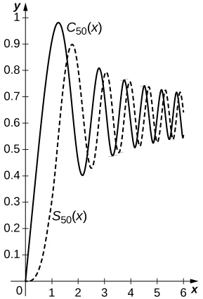
1. The Fresnel integrals are defined by \(\displaystyle C(x)=∫^x_0cos(t^2)dt\) and \(\displaystyle S(x)=∫^x_0sin(t^2)dt\). Compute the power series of \(\displaystyle C(x)\) and \(\displaystyle S(x)\) and plot the sums \(\displaystyle C_N(x)\) and \(\displaystyle S_N(x)\) of the first \(\displaystyle N=50\) nonzero terms on \(\displaystyle [0,2π]\).

Answer

Since \(\displaystyle cos(t^2)=\sum_{n=0}^∞(−1)^n\frac{t^{4n}}{(2n)!}\) and \(\displaystyle sin(t^2)=\sum_{n=0}^∞(−1)^n\frac{t^{4n+2}}{(2n+1)!}\), one has \(\displaystyle S(x)=_sum_{n=0}^∞(−1)^n\frac{x^{4n+3}}{(4n+3)(2n+1)!}\) and \(\displaystyle C(x)=\sum_{n=0}^∞(−1)^n\frac{x^{4n+1}}{(4n+1)(2n)!}\). The sums of the first \(\displaystyle 50\) nonzero terms are plotted below with \(\displaystyle C_{50}(x)\) the solid curve and \(\displaystyle S_{50}(x)\) the dashed curve.

2. The Fresnel integrals are used in design applications for roadways and railways and other applications because of the curvature properties of the curve with coordinates \(\displaystyle (C(t),S(t))\). Plot the curve \(\displaystyle (C_{50},S_{50})\) for \(\displaystyle 0≤t≤2π\), the coordinates of which were computed in the previous exercise.

Exercise \(\PageIndex{12}\)

1. Estimate \(\displaystyle ∫^{1/4}_0\sqrt{x−x^2}dx\) by approximating \(\displaystyle \sqrt{1−x}\) using the binomial approximation \(\displaystyle 1−\frac{x}{2}−\frac{x^2}{8}−\frac{x^3}{16}−\frac{5x^4}{2128}−\frac{7x^5}{256}\).

Answer

\(\displaystyle ∫^{1/4}_0\sqrt{x}(1−\frac{x}{2}−\frac{x^2}{8}−\frac{x^3}{16}−\frac{5x^4}{128}−\frac{7x^5}{256})dx =\frac{2}{3}2^{−3}−\frac{1}{2}\frac{2}{5}2^{−5}−\frac{1}{8}\frac{2}{7}2^{−7}−\frac{1}{16}\frac{2}{9}2^{−9}−\frac{5}{128}\frac{2}{11}2^{−11}−\frac{7}{256}\frac{2}{13}2^{−13}=0.0767732...\) whereas \(\displaystyle ∫^{1/4}_0\sqrt{x−x^2}dx=0.076773.\)

2. Use Newton’s approximation of the binomial \(\displaystyle \sqrt{1−x^2}\) to approximate \(\displaystyle π\) as follows. The circle centered at \(\displaystyle (\frac{1}{2},0)\) with radius \(\displaystyle \frac{1}{2}\) has upper semicircle \(\displaystyle y=\sqrt{x}\sqrt{1−x}\). The sector of this circle bounded by the \(\displaystyle x\)-axis between \(\displaystyle x=0\) and \(\displaystyle x=\frac{1}{2}\) and by the line joining \(\displaystyle (\frac{1}{4},\frac{\sqrt{3}}{4})\) corresponds to \(\displaystyle \frac{1}{6}\) of the circle and has area \(\displaystyle \frac{π}{24}\). This sector is the union of a right triangle with height \(\displaystyle \frac{\sqrt{3}}{4}\) and base \(\displaystyle \frac{1}{4}\) and the region below the graph between \(\displaystyle x=0\) and \(\displaystyle x=\frac{1}{4}\). To find the area of this region you can write \(\displaystyle y=\sqrt{x}\sqrt{1−x}=\sqrt{x}×(\text{binomial expansion of} \sqrt{1−x})\) and integrate term by term. Use this approach with the binomial approximation from the previous exercise to estimate \(\displaystyle π\).

3. Use the approximation \(\displaystyle T≈2π\sqrt{\frac{L}{g}}(1+\frac{k^2}{4})\) to approximate the period of a pendulum having length \(\displaystyle 10\) meters and maximum angle \(\displaystyle θ_{max}=\frac{π}{6}\) where \(\displaystyle k=sin(\frac{θ_{max}}{2})\). Compare this with the small angle estimate \(\displaystyle T≈2π\sqrt{\frac{L}{g}}\).

Answer

\(\displaystyle T≈2π\sqrt{\frac{10}{9.8}}(1+\frac{sin^2(θ/12)}{4})≈6.453\) seconds. The small angle estimate is \(\displaystyle T≈2π\sqrt{\frac{10}{9.8}≈6.347}\). The relative error is around \(\displaystyle 2\) percent.

4. Suppose that a pendulum is to have a period of \(\displaystyle 2\) seconds and a maximum angle of \(\displaystyle θ_{max}=\frac{π}{6}\). Use \(\displaystyle T≈2π\sqrt{\frac{L}{g}}(1+\frac{k^2}{4})\) to approximate the desired length of the pendulum. What length is predicted by the small angle estimate \(\displaystyle T≈2π\sqrt{\frac{L}{g}}\)?

5. Evaluate \(\displaystyle ∫^{π/2}_0sin^4θdθ\) in the approximation \(\displaystyle T=4\sqrt{\frac{L}{g}}∫^{π/2}_0(1+\frac{1}{2}k^2sin^2θ+\frac{3}{8}k^4sin^4θ+⋯)dθ\) to obtain an improved estimate for \(\displaystyle T\).

Answer

\(\displaystyle ∫^{π/2}_0sin^4θdθ=\frac{3π}{16}.\) Hence \(\displaystyle T≈2π\sqrt{\frac{L}{g}}(1+\frac{k^2}{4}+\frac{9}{256}k^4).\)

6. An equivalent formula for the period of a pendulum with amplitude \(\displaystyle θ_max\) is \(\displaystyle T(θ_{max})=2\sqrt{2}\sqrt{\frac{L}{g}}∫^{θ_{max}}_0\frac{dθ}{\sqrt{cosθ}−cos(θ_{max})}\) where \(\displaystyle L\) is the pendulum length and \(\displaystyle g\) is the gravitational acceleration constant. When \(\displaystyle θ_{max}=\frac{π}{3}\) we get \(\displaystyle \frac{1}{\sqrt{cost−1/2}}≈\sqrt{2}(1+\frac{t^2}{2}+\frac{t^4}{3}+\frac{181t^6}{720})\). Integrate this approximation to estimate \(\displaystyle T(\frac{π}{3})\) in terms of \(\displaystyle L\) and \(\displaystyle g\). Assuming \(\displaystyle g=9.806\) meters per second squared, find an approximate length \(\displaystyle L\) such that \(\displaystyle T(\frac{π}{3})=2\) seconds.