3.4: Maxima and Minima

Last updated
Save as PDF

Page ID: 204105

$ \newcommand{\vecs}[1]{\overset { \scriptstyle \rightharpoonup} {\mathbf{#1}} } $

$ \newcommand{\vecd}[1]{\overset{-\!-\!\rightharpoonup}{\vphantom{a}\smash {#1}}} $

$ \newcommand{\dsum}{\displaystyle\sum\limits} $

$ \newcommand{\dint}{\displaystyle\int\limits} $

$ \newcommand{\dlim}{\displaystyle\lim\limits} $

$ \newcommand{\id}{\mathrm{id}}$ $ \newcommand{\Span}{\mathrm{span}}$

( \newcommand{\kernel}{\mathrm{null}\,}\) $ \newcommand{\range}{\mathrm{range}\,}$

$ \newcommand{\RealPart}{\mathrm{Re}}$ $ \newcommand{\ImaginaryPart}{\mathrm{Im}}$

$ \newcommand{\Argument}{\mathrm{Arg}}$ $ \newcommand{\norm}[1]{\| #1 \|}$

$ \newcommand{\inner}[2]{\langle #1, #2 \rangle}$

$ \newcommand{\Span}{\mathrm{span}}$

$ \newcommand{\id}{\mathrm{id}}$

$ \newcommand{\Span}{\mathrm{span}}$

$ \newcommand{\kernel}{\mathrm{null}\,}$

$ \newcommand{\range}{\mathrm{range}\,}$

$ \newcommand{\RealPart}{\mathrm{Re}}$

$ \newcommand{\ImaginaryPart}{\mathrm{Im}}$

$ \newcommand{\Argument}{\mathrm{Arg}}$

$ \newcommand{\norm}[1]{\| #1 \|}$

$ \newcommand{\inner}[2]{\langle #1, #2 \rangle}$

$ \newcommand{\Span}{\mathrm{span}}$ $ \newcommand{\AA}{\unicode[.8,0]{x212B}}$

$ \newcommand{\vectorA}[1]{\vec{#1}} % arrow$

$ \newcommand{\vectorAt}[1]{\vec{\text{#1}}} % arrow$

$ \newcommand{\vectorB}[1]{\overset { \scriptstyle \rightharpoonup} {\mathbf{#1}} } $

$ \newcommand{\vectorC}[1]{\textbf{#1}} $

$ \newcommand{\vectorD}[1]{\overrightarrow{#1}} $

$ \newcommand{\vectorDt}[1]{\overrightarrow{\text{#1}}} $

$ \newcommand{\vectE}[1]{\overset{-\!-\!\rightharpoonup}{\vphantom{a}\smash{\mathbf {#1}}}} $

$ \newcommand{\vecs}[1]{\overset { \scriptstyle \rightharpoonup} {\mathbf{#1}} } $

$\newcommand{\longvect}{\overrightarrow}$

$ \newcommand{\vecd}[1]{\overset{-\!-\!\rightharpoonup}{\vphantom{a}\smash {#1}}} $

$\newcommand{\avec}{\mathbf a}$ $\newcommand{\bvec}{\mathbf b}$ $\newcommand{\cvec}{\mathbf c}$ $\newcommand{\dvec}{\mathbf d}$ $\newcommand{\dtil}{\widetilde{\mathbf d}}$ $\newcommand{\evec}{\mathbf e}$ $\newcommand{\fvec}{\mathbf f}$ $\newcommand{\nvec}{\mathbf n}$ $\newcommand{\pvec}{\mathbf p}$ $\newcommand{\qvec}{\mathbf q}$ $\newcommand{\svec}{\mathbf s}$ $\newcommand{\tvec}{\mathbf t}$ $\newcommand{\uvec}{\mathbf u}$ $\newcommand{\vvec}{\mathbf v}$ $\newcommand{\wvec}{\mathbf w}$ $\newcommand{\xvec}{\mathbf x}$ $\newcommand{\yvec}{\mathbf y}$ $\newcommand{\zvec}{\mathbf z}$ $\newcommand{\rvec}{\mathbf r}$ $\newcommand{\mvec}{\mathbf m}$ $\newcommand{\zerovec}{\mathbf 0}$ $\newcommand{\onevec}{\mathbf 1}$ $\newcommand{\real}{\mathbb R}$ $\newcommand{\twovec}[2]{\left[\begin{array}{r}#1 \\ #2 \end{array}\right]}$ $\newcommand{\ctwovec}[2]{\left[\begin{array}{c}#1 \\ #2 \end{array}\right]}$ $\newcommand{\threevec}[3]{\left[\begin{array}{r}#1 \\ #2 \\ #3 \end{array}\right]}$ $\newcommand{\cthreevec}[3]{\left[\begin{array}{c}#1 \\ #2 \\ #3 \end{array}\right]}$ $\newcommand{\fourvec}[4]{\left[\begin{array}{r}#1 \\ #2 \\ #3 \\ #4 \end{array}\right]}$ $\newcommand{\cfourvec}[4]{\left[\begin{array}{c}#1 \\ #2 \\ #3 \\ #4 \end{array}\right]}$ $\newcommand{\fivevec}[5]{\left[\begin{array}{r}#1 \\ #2 \\ #3 \\ #4 \\ #5 \\ \end{array}\right]}$ $\newcommand{\cfivevec}[5]{\left[\begin{array}{c}#1 \\ #2 \\ #3 \\ #4 \\ #5 \\ \end{array}\right]}$ $\newcommand{\mattwo}[4]{\left[\begin{array}{rr}#1 \amp #2 \\ #3 \amp #4 \\ \end{array}\right]}$ $\newcommand{\laspan}[1]{\text{Span}\{#1\}}$ $\newcommand{\bcal}{\cal B}$ $\newcommand{\ccal}{\cal C}$ $\newcommand{\scal}{\cal S}$ $\newcommand{\wcal}{\cal W}$ $\newcommand{\ecal}{\cal E}$ $\newcommand{\coords}[2]{\left\{#1\right\}_{#2}}$ $\newcommand{\gray}[1]{\color{gray}{#1}}$ $\newcommand{\lgray}[1]{\color{lightgray}{#1}}$ $\newcommand{\rank}{\operatorname{rank}}$ $\newcommand{\row}{\text{Row}}$ $\newcommand{\col}{\text{Col}}$ $\renewcommand{\row}{\text{Row}}$ $\newcommand{\nul}{\text{Nul}}$ $\newcommand{\var}{\text{Var}}$ $\newcommand{\corr}{\text{corr}}$ $\newcommand{\len}[1]{\left|#1\right|}$ $\newcommand{\bbar}{\overline{\bvec}}$ $\newcommand{\bhat}{\widehat{\bvec}}$ $\newcommand{\bperp}{\bvec^\perp}$ $\newcommand{\xhat}{\widehat{\xvec}}$ $\newcommand{\vhat}{\widehat{\vvec}}$ $\newcommand{\uhat}{\widehat{\uvec}}$ $\newcommand{\what}{\widehat{\wvec}}$ $\newcommand{\Sighat}{\widehat{\Sigma}}$ $\newcommand{\lt}{<}$ $\newcommand{\gt}{>}$ $\newcommand{\amp}{&}$ $\definecolor{fillinmathshade}{gray}{0.9}$

3.4 Maxima and Minima

Learning Objectives

Explain the difference between absolute and local extrema, identifying how they relate to the global behavior and local behavior of a function.
Determine the critical points of a function over a closed interval and use them, along with the endpoints of the interval, to identify absolute and local extreme values.

Definition $\PageIndex{3}$

Let $ c $ be a number in the domain $ D $ of a function $ f $. Then:

$ f(c) $ is the absolute maximum value of $ f $ on $ D $ if $ f(c) \geq f(x) \quad \text{for all } x \in D$
$ f(c) $ is the absolute minimum value of $ f $ on $ D $ if $ f(c) \leq f(x) \quad \text{for all } x \in D $

$This figure has six parts a, b, c, d, e, and f. In figure a, the line f(x) = x^3 is shown, and it is noted that it has no absolute minimum and no absolute maximum. In figure b, the line f(x) = 1/(x^2 + 1) is shown, which is near 0 for most of its length and rises to a bump at (0, 1); it has no absolute minimum, but does have an absolute maximum of 1 at x = 0. In figure c, the line f(x) = cos x is shown, which has absolute minimums of −1 at ±π, ±3π, … and absolute maximums of 1 at 0, ±2π, ±4π, …. In figure d, the piecewise function f(x) = 2 – x^2 for 0 ≤ x < 2 and x – 3 for 2 ≤ x ≤ 4 is shown, with absolute maximum of 2 at x = 0 and no absolute minimum. In figure e, the function f(x) = (x – 2)2 is shown on [1, 4], which has absolute maximum of 4 at x = 4 and absolute minimum of 0 at x = 2. In figure f, the function f(x) = x/(2 − x) is shown on [0, 2), with absolute minimum of 0 at x = 0 and no absolute maximum.$

Figure $\PageIndex{4}$: Graphs showing several possibilities for absolute extrema for functions with a domain that is a bounded interval. From OpenStax Calculus Volume 1, licensed under CC-BY-NC-SA.

Example $\PageIndex{6}$

Use the graph of $ y = f(x) $ below to find the absolute minimum and maximum values (if any).

$P16.png$

Figure $\PageIndex{5}$. A function to find absolute maximum and minimum values

Theorem $\PageIndex{3}$ The Extreme Value Theorem

Suppose that $ f $ is continuous on the closed interval $ [a, b] $. Then $ f $ attains both an absolute maximum value $ f(c) $ and an absolute minimum value $ f(d) $ at some numbers $ c $ and $ d $ in $ [a, b] $.

Definition $\PageIndex{4}$

Let $ c $ be a number in the domain $ D $ of a function $ f $. Then:

$ f(c) $ is a local maximum value of $ f $ if $ f(c) \geq f(x) \quad \text{for all } x \text{ near } c$
$ f(c) $ is a local minimum value of $ f $ if $ f(c) \leq f(x) \quad \text{for all } x \text{ near } c$

The maximum and minimum values of $ f $ are called local extreme values of $ f $.

Example $\PageIndex{7}$

Find local extreme values from the graph above (Figure 3.5)

Definition $\PageIndex{5}$

A critical number of a function $ f $ is a number $ c $ in the domain of $ f $ such that either $ f'(c) = 0 \quad \text{or} \quad f'(c) \text{ does not exist.}$ The point $ (c, f(c)) $ is called a critical point of $ f $.

Theorem $\PageIndex{4}$ Fermat's Theorem

Suppose that $ f $ has a local maximum or minimum at $ c $. If $ f'(c) $ exists, then $ f'(c) = 0$

Note

If $ f $ has a local maximum or minimum at $ c $, then $ c $ is a critical number of $ f $.

$This figure has five parts a, b, c, d, and e. In figure a, a parabola is shown facing down in quadrant I; there is a horizontal tangent line at the local maximum marked f’(c) = 0. In figure b, there is a function drawn with an asymptote at c, meaning that the function increases toward infinity on both sides of c; it is noted that f’(c) is undefined. In figure c, a version of the absolute value graph is shown that has been shifted so that its minimum is in quadrant I with x = c. It is noted that f’(c) is undefined. In figure d, a version of the function f(x) = x^3 is shown that has been shifted so that its inflection point is in quadrant I with x = c. Its inflection point at (c, f(c)) has a horizontal line through it, and it is noted that f’(c) = 0. In figure e, a version of the function f(x) = x1/3 is shown that has been shifted so that its inflection point is in quadrant I with x = c. Its inflection point at (c, f(c)) has a vertical line through it, and it is noted that f’(c) is undefined.$

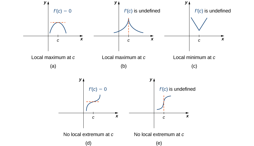
Figure $\PageIndex{6}$: Functions illustrating possible local extreme values. From OpenStax Calculus Volume 1, licensed under CC-BY-NC-SA.

Example $\PageIndex{8}$

For the functions below, find all critical numbers.

$ y= x^3 - 6x^2 + 9x + 5 $
$ y = 2(x^2 - 4)^3 $
$ y = (4x - 4)e^{-2x} $
$ y = \dfrac{x + 5}{x^2 - 9} $

The Closed Interval Method:

If we want to find the absolute maximum and minimum values of a continuous function $ f $ on a closed interval $ [a, b] $, we can follow these steps:

Find the critical numbers of $ f $ in the open interval $ (a, b) $.
Evaluate $ f $ at each critical number found in Step 1.
Evaluate $ f $ at the endpoints of the interval: $ x = a $ and $ x = b $.
The largest of the values from Steps 2 and 3 is the absolute maximum value. The smallest of these values is the absolute minimum value.

Example $\PageIndex{9}$

For each of the following functions, find the absolute maximum and absolute minimum over the specified interval. State the values and where they occur.

$ y = x^3 - 6x^2 + 9x + 5 $ over the interval $ [-1, 5] $
$ y = 2x - 4\sin x $ over the interval $ [0, \pi] $
$ y =13\ln x-14\sqrt{x}+10$ over the interval $[2, 9]$

Search

Text Color

Text Size

Margin Size

Font Type

Learning Objectives

Definition \(\PageIndex{3}\)

Example \(\PageIndex{6}\)

Theorem \(\PageIndex{3}\) The Extreme Value Theorem

Definition \(\PageIndex{4}\)

Example \(\PageIndex{7}\)

Definition \(\PageIndex{5}\)

Theorem \(\PageIndex{4}\) Fermat's Theorem

Note

Example \(\PageIndex{8}\)

Example \(\PageIndex{9}\)