4.7E: Exercises for Section 4.7

Last updated
Save as PDF

Page ID: 149910

Karen Cliffe
Southwestern College

$ \newcommand{\vecs}[1]{\overset { \scriptstyle \rightharpoonup} {\mathbf{#1}} } $

$ \newcommand{\vecd}[1]{\overset{-\!-\!\rightharpoonup}{\vphantom{a}\smash {#1}}} $

$ \newcommand{\dsum}{\displaystyle\sum\limits} $

$ \newcommand{\dint}{\displaystyle\int\limits} $

$ \newcommand{\dlim}{\displaystyle\lim\limits} $

$ \newcommand{\id}{\mathrm{id}}$ $ \newcommand{\Span}{\mathrm{span}}$

( \newcommand{\kernel}{\mathrm{null}\,}\) $ \newcommand{\range}{\mathrm{range}\,}$

$ \newcommand{\RealPart}{\mathrm{Re}}$ $ \newcommand{\ImaginaryPart}{\mathrm{Im}}$

$ \newcommand{\Argument}{\mathrm{Arg}}$ $ \newcommand{\norm}[1]{\| #1 \|}$

$ \newcommand{\inner}[2]{\langle #1, #2 \rangle}$

$ \newcommand{\Span}{\mathrm{span}}$

$ \newcommand{\id}{\mathrm{id}}$

$ \newcommand{\Span}{\mathrm{span}}$

$ \newcommand{\kernel}{\mathrm{null}\,}$

$ \newcommand{\range}{\mathrm{range}\,}$

$ \newcommand{\RealPart}{\mathrm{Re}}$

$ \newcommand{\ImaginaryPart}{\mathrm{Im}}$

$ \newcommand{\Argument}{\mathrm{Arg}}$

$ \newcommand{\norm}[1]{\| #1 \|}$

$ \newcommand{\inner}[2]{\langle #1, #2 \rangle}$

$ \newcommand{\Span}{\mathrm{span}}$ $ \newcommand{\AA}{\unicode[.8,0]{x212B}}$

$ \newcommand{\vectorA}[1]{\vec{#1}} % arrow$

$ \newcommand{\vectorAt}[1]{\vec{\text{#1}}} % arrow$

$ \newcommand{\vectorB}[1]{\overset { \scriptstyle \rightharpoonup} {\mathbf{#1}} } $

$ \newcommand{\vectorC}[1]{\textbf{#1}} $

$ \newcommand{\vectorD}[1]{\overrightarrow{#1}} $

$ \newcommand{\vectorDt}[1]{\overrightarrow{\text{#1}}} $

$ \newcommand{\vectE}[1]{\overset{-\!-\!\rightharpoonup}{\vphantom{a}\smash{\mathbf {#1}}}} $

$ \newcommand{\vecs}[1]{\overset { \scriptstyle \rightharpoonup} {\mathbf{#1}} } $

$\newcommand{\longvect}{\overrightarrow}$

$ \newcommand{\vecd}[1]{\overset{-\!-\!\rightharpoonup}{\vphantom{a}\smash {#1}}} $

$\newcommand{\avec}{\mathbf a}$ $\newcommand{\bvec}{\mathbf b}$ $\newcommand{\cvec}{\mathbf c}$ $\newcommand{\dvec}{\mathbf d}$ $\newcommand{\dtil}{\widetilde{\mathbf d}}$ $\newcommand{\evec}{\mathbf e}$ $\newcommand{\fvec}{\mathbf f}$ $\newcommand{\nvec}{\mathbf n}$ $\newcommand{\pvec}{\mathbf p}$ $\newcommand{\qvec}{\mathbf q}$ $\newcommand{\svec}{\mathbf s}$ $\newcommand{\tvec}{\mathbf t}$ $\newcommand{\uvec}{\mathbf u}$ $\newcommand{\vvec}{\mathbf v}$ $\newcommand{\wvec}{\mathbf w}$ $\newcommand{\xvec}{\mathbf x}$ $\newcommand{\yvec}{\mathbf y}$ $\newcommand{\zvec}{\mathbf z}$ $\newcommand{\rvec}{\mathbf r}$ $\newcommand{\mvec}{\mathbf m}$ $\newcommand{\zerovec}{\mathbf 0}$ $\newcommand{\onevec}{\mathbf 1}$ $\newcommand{\real}{\mathbb R}$ $\newcommand{\twovec}[2]{\left[\begin{array}{r}#1 \\ #2 \end{array}\right]}$ $\newcommand{\ctwovec}[2]{\left[\begin{array}{c}#1 \\ #2 \end{array}\right]}$ $\newcommand{\threevec}[3]{\left[\begin{array}{r}#1 \\ #2 \\ #3 \end{array}\right]}$ $\newcommand{\cthreevec}[3]{\left[\begin{array}{c}#1 \\ #2 \\ #3 \end{array}\right]}$ $\newcommand{\fourvec}[4]{\left[\begin{array}{r}#1 \\ #2 \\ #3 \\ #4 \end{array}\right]}$ $\newcommand{\cfourvec}[4]{\left[\begin{array}{c}#1 \\ #2 \\ #3 \\ #4 \end{array}\right]}$ $\newcommand{\fivevec}[5]{\left[\begin{array}{r}#1 \\ #2 \\ #3 \\ #4 \\ #5 \\ \end{array}\right]}$ $\newcommand{\cfivevec}[5]{\left[\begin{array}{c}#1 \\ #2 \\ #3 \\ #4 \\ #5 \\ \end{array}\right]}$ $\newcommand{\mattwo}[4]{\left[\begin{array}{rr}#1 \amp #2 \\ #3 \amp #4 \\ \end{array}\right]}$ $\newcommand{\laspan}[1]{\text{Span}\{#1\}}$ $\newcommand{\bcal}{\cal B}$ $\newcommand{\ccal}{\cal C}$ $\newcommand{\scal}{\cal S}$ $\newcommand{\wcal}{\cal W}$ $\newcommand{\ecal}{\cal E}$ $\newcommand{\coords}[2]{\left\{#1\right\}_{#2}}$ $\newcommand{\gray}[1]{\color{gray}{#1}}$ $\newcommand{\lgray}[1]{\color{lightgray}{#1}}$ $\newcommand{\rank}{\operatorname{rank}}$ $\newcommand{\row}{\text{Row}}$ $\newcommand{\col}{\text{Col}}$ $\renewcommand{\row}{\text{Row}}$ $\newcommand{\nul}{\text{Nul}}$ $\newcommand{\var}{\text{Var}}$ $\newcommand{\corr}{\text{corr}}$ $\newcommand{\len}[1]{\left|#1\right|}$ $\newcommand{\bbar}{\overline{\bvec}}$ $\newcommand{\bhat}{\widehat{\bvec}}$ $\newcommand{\bperp}{\bvec^\perp}$ $\newcommand{\xhat}{\widehat{\xvec}}$ $\newcommand{\vhat}{\widehat{\vvec}}$ $\newcommand{\uhat}{\widehat{\uvec}}$ $\newcommand{\what}{\widehat{\wvec}}$ $\newcommand{\Sighat}{\widehat{\Sigma}}$ $\newcommand{\lt}{<}$ $\newcommand{\gt}{>}$ $\newcommand{\amp}{&}$ $\definecolor{fillinmathshade}{gray}{0.9}$

For exercises 1 - 2, determine the area of the region between the two curves in the given figure by integrating over the $x$-axis.

1) $y=x^2−3$ and $y=1$

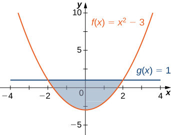
$This figure is has two graphs. They are the functions f(x) = x^2-3and g(x)=1. In between these graphs is a shaded region, bounded above by g(x) and below by f(x). The shaded area is between x=-2 and x=2.$

Answer: $\dfrac{32}{3} \, \text{units}^2$

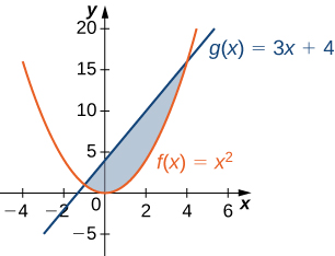
2) $y=x^2$ and $y=3x+4$

$This figure is has two graphs. They are the functions f(x) = x^2 and g(x)= 3x+4. In between these graphs is a shaded region, bounded above by g(x) and below by g(x).$

For exercise 3, split the region between the two curves into two smaller regions, then determine the area by integrating over the $x$-axis. Note that you will have two integrals to solve.

3) $y=x^3$ and $ y=x^2+x$

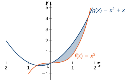
$This figure is has two graphs. They are the functions f(x) = x^3 and g(x)= x^2+x. These graphs intersect twice. The regions between the intersections are shaded. The first region is bounded above by f(x) and below by g(x). The second region is bounded above by g(x) and below by f(x).$

Answer: $\dfrac{13}{12}\, \text{units}^2$

For exercises 4-5, determine the area of the region between the two curves by integrating over the $y$-axis.

4) $x=y^2$ and $x=9$

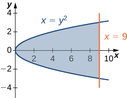
$This figure is has two graphs. They are the equations x=y^2 and x=9. The region between the graphs is shaded. It is horizontal, between the y-axis and the line x=9.$

Answer: $36 \, \text{units}^2$

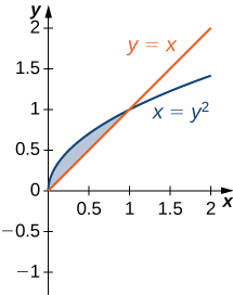
5) $y=x$ and $ x=y^2$

$This figure is has two graphs. They are the equations y=x and x=y^2. The region between the graphs is shaded, bounded above by x=y^2 and below by y=x.$

For exercises 6-12, graph the equations and shade the area of the region between the curves. Determine its area by integrating over the $x$-axis.

6) $y=x^2$ and $y=−x^2+18x$

Answer

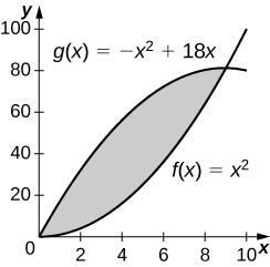
$This figure is has two graphs. They are the functions f(x)=x^2 and g(x)=-x^2+18x. The region between the graphs is shaded, bounded above by g(x) and below by f(x). It is in the first quadrant.$

243 square units

7) $y=\dfrac{1}{x}, \quad y=\dfrac{1}{x^2}$, and $x=3$

8) $y=\sqrt{x}$ and $y=x^2$

Answer

$clipboard_ec14483ed82e91a2332bafc858209e569.png$

1/3 square units

9) $y=e^x,\quad y=e^{2x−1}$, and $x=0$

10) $y=e^x, \quad y=e^{−x}, \quad x=−1$ and $x=1$

Answer

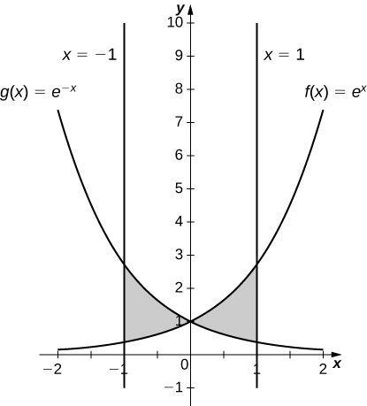
$This figure is has two graphs. They are the functions f(x)=e^x and g(x)=e^-x. There are two shaded regions. In the second quadrant the region is bounded by x=-1, g(x) above and f(x) below. The second region is in the first quadrant and is bounded by f(x) above, g(x) below, and x=1.$

$\dfrac{2(e−1)^2}{e}\, \text{units}^2$

11) $ y=e, \quad y=e^x,$ and $y=e^{−x}$

12) $y=|x|$ and $y=x^2$

Answer

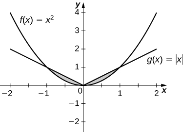
$This figure is has two graphs. They are the functions f(x)=x^2 and g(x)=absolute value of x. There are two shaded regions. The first region is in the second quadrant and is between g(x) above and f(x) below. The second region is in the first quadrant and is bounded above by g(x) and below by f(x).$

$\dfrac{1}{3}\, \text{units}^2$

For exercises 13-18, graph the equations and shade the area of the region between the curves. If necessary, break the region into sub-regions to determine its entire area.

13) $y=8-2x,\quad y=x,$ and $y=0$

14) $y=12−x,\quad y=\sqrt{x},$ and $y=1$

Answer

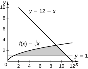
$This figure is has three graphs. They are the functions f(x)=squareroot of x, y=12-x, and y=1. The region between the graphs is shaded, bounded above and to the left by f(x), above and to the right by the line y=12-x, and below by the line y=1. It is in the first quadrant.$

$\dfrac{34}{3}\, \text{units}^2$

15) $y=x^2$ and $y=\frac{8}{x}$ and $y=1$

16) $y=x^3$ and $y=x^2−2x$ over $x \in [−1,1]$

Answer

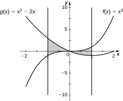
$This figure is has two graphs. They are the functions f(x)=x^3 and g(x)=x^2-2x. There are two shaded regions between the graphs. The first region is bounded to the left by the line x=-2, above by g(x) and below by f(x). The second region is bounded above by f(x), below by g(x) and to the right by the line x=2.$

$\dfrac{5}{2}\, \text{units}^2$

17) $y=x^2+9$ and $ y=10+2x$ over $x \in [−1,3]$

18) $y=x^3+3x$ and $y=4x$

Answer

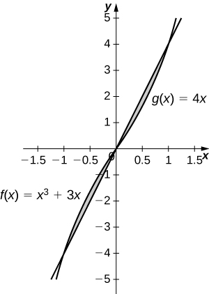
$This figure is has two graphs. They are the functions f(x)=x^3+3x and g(x)=4x. There are two shaded regions between the graphs. The first region is bounded above by f(x) and below by g(x). The second region is bounded above by g(x), below by f(x).$

$\dfrac{1}{2}\, \text{units}^2$

For exercises 19-22, graph the equations and shade the area of the region between the curves. Determine its area by integrating over the $y$-axis.

19) $x=y^3$ and $ x = 3y−2$

20) $x=y$ and $ x=y^3−y$

Answer

$This figure is has two graphs. They are the equations x=2y and x=y^3-y. The graphs intersect in the third quadrant and again in the first quadrant forming two closed regions in between them.$

$\dfrac{9}{2}\, \text{units}^2$

21) $x=−3+y^2$ and $ x=y−y^2$

22) $y^2=x$ and $x=y+2$

Answer

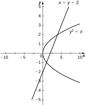
$This figure is has two graphs. They are the equations x=y+2 and y^2=x. The graphs intersect, forming a region in between them$

$\dfrac{9}{2}\, \text{units}^2$

For exercises 23-29, graph the equations and shade the area of the region between the curves. Determine its area by integrating over the $x$-axis or $y$-axis, whichever seems more convenient.

23) $x=y^4$ and $x=y^5$

24) $y=x^6$ and $y=x^4$

25) $x=y^3+2y^2+1$ and $x=−y^2+1$

Answer

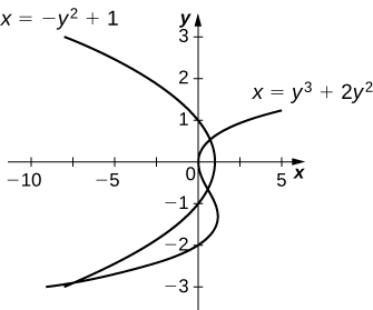
$This figure is has two graphs. They are the equations x=-y^2+1 and x=y^3+2y^2. The graphs intersect, forming two regions in between them.$

$\dfrac{27}{4}\, \text{units}^2$

26) $ y=|x|$ and $ y=x^2−1$

27) $y=4−3x$ and $y=\dfrac{1}{x}$

Answer

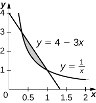
$This figure is has two graphs. They are the equations y=4-3x and y=1/x. The graphs intersect, having region between them shaded. The region is in the first quadrant.$

$\left(\dfrac{4}{3}−\ln(3)\right)\, \text{units}^2$

28) $y=x^2−3x+2$ and $ y=x^3−2x^2−x+2$

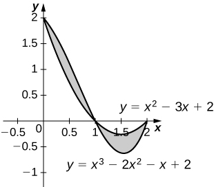
Answer: $This figure is has two graphs. They are the equations y=x^2-3x+2 and y=x^3-2x^2-x+2. The graphs intersect, having region between them shaded.$
$\dfrac{1}{2}$ square units

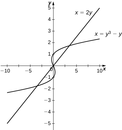
29) $y+y^3=x$ and $2y=x$

Answer

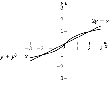
$This figure is has two graphs. They are the equations 2y=x and y+y^3=x. The graphs intersect, forming two regions. The regions are shaded.$

$\dfrac{1}{2}$ square units

30) A factory selling cell phones has a marginal cost function $C(x)=0.01x^2−3x+229$, where $x$ represents the number of cell phones, and a marginal revenue function given by $R(x)=429−2x.$ Find the area between the graphs of these curves and $x=0.$ What does this area represent?

Answer: $33,333.33 total profit for 200 cell phones sold

31) An amusement park has a marginal cost function $C(x)=1000e−x+5$, where $x$ represents the number of tickets sold, and a marginal revenue function given by $R(x)=60−0.1x$. Find the total profit generated when selling $550$ tickets. Use a calculator to determine intersection points, if necessary, to two decimal places.

Contributors

Gilbert Strang (MIT) and Edwin “Jed” Herman (Harvey Mudd) with many contributing authors. This content by OpenStax is licensed with a CC-BY-SA-NC 4.0 license. Download for free at http://cnx.org.

Search

Text Color

Text Size

Margin Size

Font Type