4.4E: Exercises for Section 4.4

1) Consider two athletes running at variable speeds \(v_1(t)\) and \(v_2(t).\) The runners start and finish a race at exactly the same time. Explain why the two runners must be going the same speed at some point.

2) Two mountain climbers start their climb at base camp, taking two different routes, one steeper than the other, and arrive at the peak at exactly the same time. Is it necessarily true that, at some point, both climbers increased in altitude at the same rate?

Answer

Yes. It is implied by the Mean Value Theorem for Integrals.

3) To get on a certain toll road a driver has to take a card that lists the mile entrance point. The card also has a timestamp. When going to pay the toll at the exit, the driver is surprised to receive a speeding ticket along with the toll. Explain how this can happen.

4) Set \(\displaystyle F(x)=∫^x _1(1−t)\,dt.\) Find \( F′(2)\) and the average value of \(F'\) over \([1,2].\)

Answer

\(F′(2)=−1;\) average value of \(F'\) over \( [1,2]\) is \(−1/2.\)

In exercises 5 - 16, use the Fundamental Theorem of Calculus, Part 1, to find each derivative.

5) \(\displaystyle \frac{d}{dx}\left[∫^x_1e^{−t^2}\,dt \right] \)

6) \(\displaystyle \frac{d}{dx}\left[∫^x_1e^{cost}\,dt \right] \)

Answer

\(\displaystyle \frac{d}{dx}\left[∫^x_1e^{cost}\,dt \right] = e^{\cos t}\)

7) \(\displaystyle \frac{d}{dx}\left[∫^x_3\sqrt{9−y^2}\,dy \right] \)

8) \(\displaystyle \frac{d}{dx}\left[∫^x_3\frac{ds}{\sqrt{16−s^2}} \right] \)

Answer

\(\displaystyle \frac{d}{dx}\left[∫^x_3\frac{ds}{\sqrt{16−s^2}} \right] = \frac{1}{\sqrt{16−x^2}}\)

9) \(\displaystyle \frac{d}{dx}\left[∫^{2x}x_t\,dt \right] \)

10) \(\displaystyle \frac{d}{dx}\left[∫^{\sqrt{x}}_0t\,dt \right] \)

Answer

\(\displaystyle \frac{d}{dx}\left[∫^{\sqrt{x}}_0t\,dt \right] = \sqrt{x}\frac{d}{dx}\big(\sqrt{x}\big)=\frac{1}{2}\)

11) \(\displaystyle \frac{d}{dx}\left[∫^{\sin x}_0\sqrt{1−t^2}\,dt \right] \)

12) \(\displaystyle \frac{d}{dx}\left[∫^1_{\cos x}\sqrt{1−t^2}\,dt \right] \)

Answer

\(\displaystyle \frac{d}{dx}\left[∫^1_{\cos x}\sqrt{1−t^2}\,dt \right] = −\sqrt{1−\cos^2x}\frac{d}{dx}\big(\cos x\big)=|\sin x|\sin x\)

13) \(\displaystyle \frac{d}{dx}\left[∫^{\sqrt{x}}_1\frac{t^2}{1+t^4}\,dt \right] \)

14) \(\displaystyle \frac{d}{dx}\left[∫^{x^2}_1\frac{\sqrt{t}}{1+t}\,dt \right] \)

Answer

\(\displaystyle \frac{d}{dx}\left[∫^{x^2}_1\frac{\sqrt{t}}{1+t}\,dt \right] = 2x\dfrac{|x|}{1+x^2}\)

15) \(\displaystyle \frac{d}{dx}\left[∫^{\ln x}_0e^t\,dt \right] \)

16) \(\displaystyle \frac{d}{dx}\left[∫^{e^{x}}_1\ln u^2\,du \right] \)

Answer

\(\displaystyle \frac{d}{dx} \left[ ∫^{e^{x}}_1\ln u^2\,du \right] = \ln(e^{2x})\dfrac{d}{dx}\big(e^x\big)=2xe^x\)

17) The graph of \(\displaystyle y=∫^x_0f(t)\,dt\), where \(f\) is a piecewise constant function, is shown here.

a. Over which intervals is \(f\) positive? Over which intervals is it negative? Over which intervals, if any, is it equal to zero?

b. What are the maximum and minimum values of \(f\)?

c. What is the average value of \(f\)?

18) The graph of \(\displaystyle y=∫^x_0f(t)\,dt\), where \(f\) is a piecewise constant function, is shown here.

a. Over which intervals is \(f\) positive? Over which intervals is it negative? Over which intervals, if any, is it equal to zero?

b. What are the maximum and minimum values of \(f\)?

c. What is the average value of \(f\)?

Answer

a. \(f\) is positive over \([1,2]\) and \([5,6]\), negative over \( [0,1]\) and \([3,4]\), and zero over \([2,3]\) and \([4,5]\).
b. The maximum value is \(2\) and the minimum is \(−3\).
c. The average value is \(0\).

19) The graph of \(\displaystyle y=∫^x_0ℓ(t)\,dt\), where \(ℓ\) is a piecewise linear function, is shown here.

a. Over which intervals is \(ℓ\) positive? Over which intervals is it negative? Over which, if any, is it zero?

b. Over which intervals is \(ℓ\) increasing? Over which is it decreasing? Over which, if any, is it constant?

c. What is the average value of \(ℓ\)?

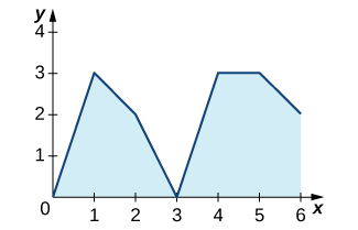
20) The graph of \(\displaystyle y=∫^x_0ℓ(t)\,dt\), where \( ℓ\) is a piecewise linear function, is shown here.

a. Over which intervals is \(ℓ\) positive? Over which intervals is it negative? Over which, if any, is it zero?

b. Over which intervals is \(ℓ\) increasing? Over which is it decreasing? Over which intervals, if any, is it constant?

c. What is the average value of \(ℓ\)?

Answer

a. \(ℓ\) is positive over \([0,1]\) and \([3,6]\), and negative over \([1,3]\).
b. It is increasing over \([0,1]\) and \([3,5]\), and it is constant over \([1,3]\) and \([5,6]\).
c. Its average value is \(\dfrac{1}{3}\).

In exercises 21 - 26, use a calculator to estimate the area under the curve by computing \( T_{10}\), the average of the left- and right-endpoint Riemann sums using \(N=10\) rectangles. Then, using the Fundamental Theorem of Calculus, Part 2, determine the exact area.

21) [T] \( y=x^2\) over \( [0,4]\)

22) [T] \(y=x^3+6x^2+x−5\) over \( [−4,2]\)

Answer

\(\displaystyle T_{10}=49.08,\quad ∫^3_{−2}\left(x^3+6x^2+x−5\right)\,dx=48\)

23) [T] \(y=\sqrt{x^3}\) over \( [0,6]\)

24) [T] \(y=\sqrt{x}+x^2\) over \([1,9]\)

Answer

\(\displaystyle T_{10}=260.836,\quad ∫^9_1(\sqrt{x}+x^2)\,dx=260\)

25) [T] \(\displaystyle ∫(e^x)\,dx\) over \(\displaystyle [0,2]\)

26) [T] \(\displaystyle ∫\frac{4}{x^2}\,dx\) over \(\displaystyle [1,4]\)

Answer

\(\displaystyle T_{10}=3.058,\quad ∫^4_1\frac{4}{x^2}\,dx=3\)

In exercises 27 - 40, evaluate each definite integral using the Fundamental Theorem of Calculus, Part 2.

27) \(\displaystyle ∫^2_{−1}(x^2−3x)\,dx\)

28) \(\displaystyle ∫^3_{−2}(x^2+3x−5)\,dx\)

Answer

\(\displaystyle F(x)=\frac{x^3}{3}+\frac{3x^2}{2}−5x,\quad F(3)−F(−2)=−\frac{35}{6}\)

29) \(\displaystyle ∫^3_{−2}(t+2)(t−3)dt\)

30) \(\displaystyle ∫^3_2(t^2−9)(4−t^2)dt\)

Answer

\(F(x)=−\dfrac{t^5}{5}+\dfrac{13t^3}{3}−36t,\quad F(3)−F(2)=\frac{62}{15}\)

31) \(\displaystyle ∫^2_1x^9\,dx\)

32) \(\displaystyle ∫^1_0x^{99}\,dx\)

Answer

\(F(x)=\dfrac{x^{100}}{100},\quad F(1)−F(0)=\dfrac{1}{100}\)

33) \(\displaystyle ∫^8_4(4t^{5/2}−3t^{3/2})dt\)

34) \(\displaystyle ∫^4_{1/4}\left(x^2−\dfrac{1}{x^2}\right)\,dx\)

Answer

\(F(x)=\dfrac{x^3}{3}+\dfrac{1}{x},\quad F(4)−F\left(\tfrac{1}{4}\right)=\frac{1125}{64}\)

35) \(\displaystyle ∫^2_1\frac{2}{x^3}\,dx\)

36) \(\displaystyle ∫^4_1\frac{1}{2\sqrt{x}}\,dx\)

Answer

\(F(x)=\sqrt{x},\quad F(4)−F(1)=1\)

37) \(\displaystyle ∫^4_1\frac{2−\sqrt{t}}{t^2}\,dt\)

38) \(\displaystyle ∫^{16}_1\frac{dt}{t^{1/4}}\)

Answer

\( F(t)=\frac{4}{3}t^{3/4},\quad F(16)−F(1)=\frac{28}{3}\)

39) \(\displaystyle ∫^2_1\left(\frac{1}{t^2}−\frac{1}{t^3}\right)\,dt\)

40) \(\displaystyle ∫^{−1}_{−2}\left(\frac{1}{t^2}−\frac{1}{t^3}\right)\,dt\)

Answer

\( F(t)=−\dfrac{1}{t}+\dfrac{1}{2t^2},\quad F(−1)−F(−2)=\frac{7}{8}\)

In exercises 41-42, use the evaluation theorem to express the integral as a function \(F(x)\).

41) \(\displaystyle ∫^x_at^2\,dt\)

42) \(\displaystyle ∫^x_1e^t\,dt\)

Answer

\(F(x)=e^x−e\)

In exercises 43-44, identify the roots of the integrand to remove absolute values, then evaluate using the Fundamental Theorem of Calculus, Part 2.

43) \(\displaystyle ∫^3_{−2}|x|\,dx\)

44) \(\displaystyle ∫^4_{−2}∣t^2−2t−3∣\,dt\)

Answer

\(\displaystyle ∫^{−1}_{−2}(t^2−2t−3)\,dt−∫^3_{−1}(t^2−2t−3)\,dt+∫^4_3(t^2−2t−3)\,dt=\frac{46}{3}\)

45) Suppose that for a particular company, the spending on construction projects between 2010 (\(t=1\)) to 2019 (\(t=20\)) is modeled by the function \(S(t)=25\sqrt{t}\), where \(S\) is measured in thousands of dollars per year and \(t\) is measured in years. What is the average spending per year on construction projects between 2010 and 2019?

46) Suppose the rate of gasoline consumption for a family over a one year period (\(t=0\) to \(t=12\)) can be modeled by the function \(-t^2+12t+25\) gal/mo.What is the average monthly consumption, and for which value(s) of \(t\) is the rate at time \(t\) equal to the average rate?

Answer

The average value is 49 gal/mo, and the rate is equal to the average value at approximately time \(t=2.54\) and \(t=9.46\).

47) Explain why, if \(f\) is continuous over \([a,b],\) there is at least one point \( c∈[a,b]\) such that \(\displaystyle f(c)=\frac{1}{b−a}∫^b_af(t)\,dt.\)

48) Explain why, if \(f\) is continuous over \([a,b]\) and is not equal to a constant, there is at least one point \( M∈[a,b]\) such that \(\displaystyle f(M)=\frac{1}{b−a}∫^b_af(t)\,dt\) and at least one point \(m∈[a,b]\) such that \(\displaystyle f(m)<\frac{1}{b−a}∫^b_af(t)\,dt\).

Answer

If \(f\) is not constant, then its average is strictly smaller than the maximum and larger than the minimum, which are attained over \([a,b]\) by the extreme value theorem.