
12.3: Mean-Field Approximation


- Last updated
- Apr 30, 2024
- Save as PDF

( \newcommand{\kernel}{\mathrm{null}\,}\)
Behaviors of CA models are complex and highly nonlinear, so it isn’t easy to analyze their dynamics in a mathematically elegant way. But still, there are some analytical methods available. Mean-field approximation is one such analytical method. It is a powerful analytical method to make a rough prediction of the macroscopic behavior of a complex system. It is widely used to study various kinds of large-scale dynamical systems, not just CA. Having said that, it is often misleading for studying complex systems (this issue will be discussed later), but as a first step of mathematical analysis, it isn’t so bad either.
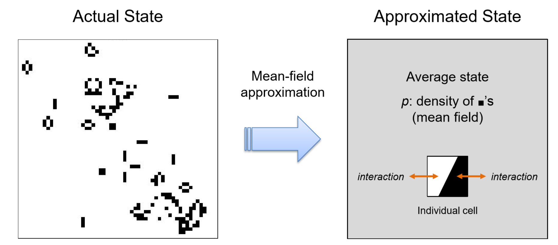
In any case, the primary reason why it is so hard to analyze CA and other complex systems is that they have a large number of dynamical variables. Mean-field approximation drastically reduces this high dimensionality down to just a few dimensions (!) by reformulating the dynamics of the system in terms of the “average state” of the system (Fig.12.3.2). Then the dynamics are re-described in terms of how each individual cell interacts with this average state and how the average state itself changes over time. In so doing, it is assumed that every cell in the entire space chooses its next state independently, according to the probabilities determined by the average state of the system. This hypothetical, homogeneous, probabilistic space is called the mean field, from which the name of the approximation method was derived. Averaging the whole system is equivalent to randomizing or ignoring spatial relationships among components, so you can say that mean-field approximation is a technique to approximate spatial dynamics by non-spatial ones.
Let’s work on an example. Consider applying the mean-field approximation to a 2-D binary CA model with the majority rule on Moore neighborhoods. When we apply meanfield approximation to this model, the size of the space no longer matters, because, no
matter how large the space is, the system’s state is approximated just by one variable: the density of 1’s, pt. This is the mean field, and now our task is to describe its dynamics in a difference equation.
When we derive a new difference equation for the average state, we no longer have any specific spatial configuration; everything takes place probabilistically. Therefore, we need to enumerate all possible scenarios of an individual cell’s state transition, and then calculate the probability for each scenario to occur.
Table 12.3.1 lists all possible scenarios for the binary CA with the majority rule. The probability of each state transition event is calculated by (probability for the cell to take the “Current state”) × (probability for the eight neighbors to be in any of the “Neighbors’ states”). The latter is the sum of (number of ways to arrange k 1’s in 8 cells)×(probability for k cells to be 1)×(probability for 8−k cells to be 0) over the respective range of k. You may have learned about this kind of combinatorial calculation of probabilities in discrete mathematics and/or probability and statistics.
Confirm that the probabilities listed in the last column of Table 12.3.1 are a valid probability distribution, i.e., that the sum of them is 1.
To write a difference equation of pt, there are only two scenarios we need to take into account: the second and fourth ones in Table 12.3.1, whose next state is 1. This is
Table 12.3.1: Possible scenarios of state transitions for binary CA with the majority rule.
| Current state | Neighbors’ states | Next state | Probability of this transition |
|---|---|---|---|
| 0 | Four 1’s or fewer | 0 | (1−p)∑4k=0(8k)pk(1−p)(8−k) |
| 0 | Five 1’s or more | 1 | (1−p)∑8k=5(8k)pk(1−p)(8−k) |
| 1 | Three 1’s or fewer | 0 | p∑3k=0(8k)pk(1−p)(8−k) |
| 1 | Four 1’s or more | 1 | p∑8k=4(8k)pk(1−p)(8−k) |
because the next value of the average state, pt+1, is the probability for the next state to be 1. Therefore, we can write the following difference equation (the subscript of pt is omitted on the right hand side for simplicity):
pt+1=(1−p)8∑k=5(8k)pk(1−p)(8−k)+p8∑k=4(8k)pk(1−p)(8−k)
=8∑k=5(8k)pk(1−p)(8−k)+(84)p4(1−p)4
=(85)p5(1−p)3+(86)p6(1−p)2+(87)p7(1−p)+(88)p8+70p5(1−p)4
=56p5(1−p)3+28p6(1−p)2+8p7(1−p)+p8+70p5(1−p)4
=70p9−315p8+540p7−420p6+126p5
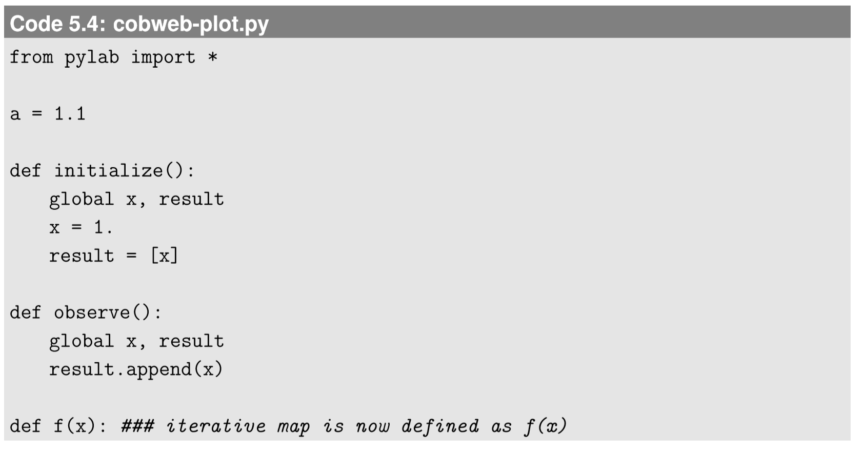
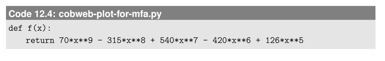
This result may still seem rather complicated, but it is now nothing more than a one-dimensional nonlinear iterative map, and we already learned how to analyze its dynamics in Chapter 5. For example, we can draw a cobweb plot of this iterative map by replacing the function f(x) in Code 5.4 with the following (you should also change xmin and xmax to see the whole picture of the cobweb plot):
This produces the cobweb plot shown in Fig. 12.3.2. This plot clearly shows that there are three equilibrium points (p=0, 1/2, and 1), p=0 and 1 are stable while p=1/2 is unstable, and the asymptotic state is determined by whether the initial value is below or above 1/2. This prediction makes some sense in view of the nature of the state-transition function (the majority rule); interaction with other individuals will bring the whole system a little closer to the majority choice, and eventually everyone will agree on one of the two choices.
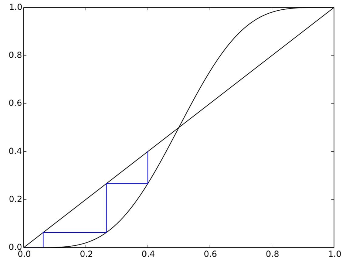
Figure 12.3.1: Cobweb plot of Equation ???.
However, we should note that the prediction made using the mean-field approximation above doesn’t always match what actually happens in spatially explicit CA models. In simulations, you often see clusters of cells with the minority state remaining in space, making it impossible for the whole system to reach a unanimous consensus. This is because, after all, mean-field approximation is no more than an approximation. It produces a prediction that holds only in an ideal scenario where the spatial locality can be ignored and every component can be homogeneously represented by a global average, which, unfortunately, doesn’t apply to most real-world spatial systems that tend to have nonhomogeneous states and/or interactions. So you should be aware of when you can apply mean-field approximation, and what are its limitations, as summarized below:
Mean-field approximation is a technique that ignores spatial relationships among components. It works quite well for systems whose parts are fully connected or randomly interacting with each other. It doesn’t work if the interactions are local or non-homogeneous, and/or if the system has a non-uniform pattern of states. In such cases, you could still use mean-field approximation as a preliminary, “zeroth-order” approximation, but you should not derive a final conclusion from it.
In some sense, mean-field approximation can serve as a reference point to understand the dynamics of your model system. If your model actually behaves the same way as predicted by the mean-field approximation, that probably means that the system is not quite complex and that its behavior can be understood using a simpler model.
Apply mean-field approximation to the Game of Life 2-D CA model. Derive a difference equation for the average state density pt, and predict its asymptotic behavior. Then compare the result with the actual density obtained from a simulation result. Do they match or not? Why?