3.2: Phase Space

Last updated
Save as PDF

Page ID: 7779

\( \newcommand{\vecs}[1]{\overset { \scriptstyle \rightharpoonup} {\mathbf{#1}} } \) \( \newcommand{\vecd}[1]{\overset{-\!-\!\rightharpoonup}{\vphantom{a}\smash {#1}}} \)\(\newcommand{\id}{\mathrm{id}}\) \( \newcommand{\Span}{\mathrm{span}}\) \( \newcommand{\kernel}{\mathrm{null}\,}\) \( \newcommand{\range}{\mathrm{range}\,}\) \( \newcommand{\RealPart}{\mathrm{Re}}\) \( \newcommand{\ImaginaryPart}{\mathrm{Im}}\) \( \newcommand{\Argument}{\mathrm{Arg}}\) \( \newcommand{\norm}[1]{\| #1 \|}\) \( \newcommand{\inner}[2]{\langle #1, #2 \rangle}\) \( \newcommand{\Span}{\mathrm{span}}\) \(\newcommand{\id}{\mathrm{id}}\) \( \newcommand{\Span}{\mathrm{span}}\) \( \newcommand{\kernel}{\mathrm{null}\,}\) \( \newcommand{\range}{\mathrm{range}\,}\) \( \newcommand{\RealPart}{\mathrm{Re}}\) \( \newcommand{\ImaginaryPart}{\mathrm{Im}}\) \( \newcommand{\Argument}{\mathrm{Arg}}\) \( \newcommand{\norm}[1]{\| #1 \|}\) \( \newcommand{\inner}[2]{\langle #1, #2 \rangle}\) \( \newcommand{\Span}{\mathrm{span}}\)\(\newcommand{\AA}{\unicode[.8,0]{x212B}}\)

Behaviors of a dynamical system can be studied by using the concept of a phase space, which is informally defined as follows:

Definition: Phase Space

A phase space of a dynamical system is a theoretical space where every state of the system is mapped to a unique spatial location.

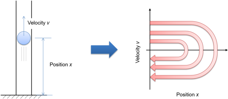
The number of state variables needed to uniquely specify the system’s state is called the degrees of freedom in the system. You can build a phase space of a system by having an axis for each degree of freedom, i.e., by taking each state variable as one of the orthogonal axes. Therefore, the degrees of freedom of a system equal the dimensions of its phase space. For example, describing the behavior of a ball thrown upward in a frictionless vertical tube can be specified with two scalar variables, the ball’s position and velocity, at least until it hits the bottom again. You can thus create its phase space in two dimensions, as shown in Fig. 3.2.1.

Figure \(\PageIndex{1}\): A ball is thrown upward in a vertical tube (left) and a scheatic illustration of its phase space (right). The dynamic behavior of the ball can be visualize as a static trajectory in the phase space (red arrows).

One of the benefits of drawing a phase space is that it allows you to visually represent the dynamically changing behavior of a system as a static trajectory in it. This provides a lot of intuitive, geometrical insight into the system’s dynamics, which would be hard to infer if you were just looking at algebraic equations.

Exercise \(\PageIndex{1}\)

In the example above, when the ball hits the ﬂoor in the vertical tube, its kinetic energy is quickly converted into elastic energy (i.e., deformation of the ball), and then it is converted back into kinetic energy again (i.e., upward velocity). Think about how you can illustrate this process in the phase space. Are the two dimensions enough or do you need to introduce an additional dimension? Then try to illustrate the trajectory of the system going through a bouncing event in the phase space.