3.2: The Mean Value Theorem

We motivate this section with the following question: Suppose you leave your house and drive to your friend's house in a city 100 miles away, completing the trip in two hours. At any point during the trip do you necessarily have to be going 50 miles per hour?

In answering this question, it is clear that the average speed for the entire trip is 50 mph (i.e. 100 miles in 2 hours), but the question is whether or not your instantaneous speed is ever exactly 50 mph. More simply, does your speedometer ever read exactly 50 mph?. The answer, under some very reasonable assumptions, is "yes."'

Let's now see why this situation is in a calculus text by translating it into mathematical symbols.

First assume that the function \(y = f(t)\) gives the distance (in miles) traveled from your home at time \(t\) (in hours) where \(0\le t\le 2\). In particular, this gives \(f(0)=0\) and \(f(2)=100\). The slope of the secant line connecting the starting and ending points \((0,f(0))\) and \((2,f(2))\) is therefore

$$
\frac{\Delta f}{\Delta t} = \frac{f(2)-f(0)}{2-0} = \frac{100-0}{2} = 50 \, \text{mph}.
\]

The slope at any point on the graph itself is given by the derivative \(f'(t)\). So, since the answer to the question above is "yes," this means that at some time during the trip, the derivative takes on the value of 50 mph. Symbolically,

$$
f'(c) = \frac{f(2)-f(0)}{2-0} = 50
\]

for some time \(0\le c \le 2.\)

How about more generally? Given any function \(y=f(x)\) and a range \(a\le x\le b\) does the value of the derivative at some point between \(a\) and \(b\) have to match the slope of the secant line connecting the points \((a,f(a))\) and \((b,f(b))\)? Or equivalently, does the equation

\[f'(c) = \frac{f(b)-f(a)}{b-a}\]

have to hold for some \(a < c < b\)?

Let's look at two functions in an example.

Example \(\PageIndex{1}\): Comparing average and instantaneous rates of change

Consider functions

$$f_1(x)=\frac{1}{x^2}\quad \text{and} \quad f_2(x) = |x|\]

with \(a=-1\) and \(b=1\) as shown in Figure \(\PageIndex{1}\) (a) and (b), respectively. Both functions have a value of 1 at \(a\) and \(b\). Therefore the slope of the secant line connecting the end points is \(0\) in each case. But if you look at the plots of each, you can see that there are no points on either graph where the tangent lines have slope zero. Therefore we have found that there is no \(c\) in \([-1,1]\) such that

$$f'(c) = \frac{f(1)-f(-1)}{1-(-1)} = 0.\]

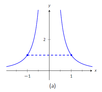
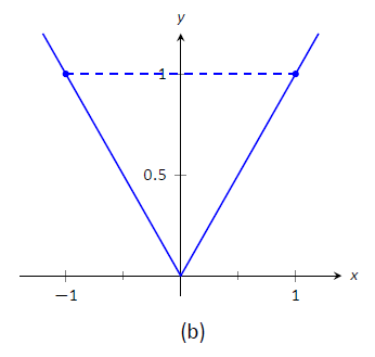
Figure \(\PageIndex{1}\): A graph of \(f_1(x) = 1/x^2\) and \(f_2(x) = |x|\) in Example \(\PageIndex{1}\).

So what went "wrong"'? It may not be surprising to find that the discontinuity of \(f_1\) and the corner of \(f_2\) play a role. If our functions had been continuous and differentiable, would we have been able to find that special value \(c\)? This is our motivation for the following theorem.

Theorem \(\PageIndex{1}\): The Mean Value Theorem of Differentiation

Let \(y=f(x)\) be continuous function on the closed interval \([a,b]\) and differentiable on the open interval \((a,b)\). There exists a value \(c\), \(a < c < b\), such that
$$
f'(c) = \frac{f(b)-f(a)}{b-a}.
$$
That is, there is a value \(c\) in \((a,b)\) where the instantaneous rate of change of \(f\) at \(c\) is equal to the average rate of change of \(f\) on \([a,b]\).

Note that the reasons that the functions in Example \(\PageIndex{1}\) fail are indeed that \(f_1\) has a discontinuity on the interval \([-1,1]\) and \(f_2\) is not differentiable at the origin.

We will give a proof of the Mean Value Theorem below. To do so, we use a fact, called Rolle's Theorem, stated here.

Theorem \(\PageIndex{2}\): Rolle's Theorem

Let \(f\) be continuous on \([a,b]\) and differentiable on \((a,b)\), where \(f(a) = f(b)\). There is some \(c\) in \((a,b)\) such that \(f'(c) = 0.\)

Consider Figure \(\PageIndex{2}\) where the graph of a function \(f\) is given, where \(f(a) = f(b)\). It should make intuitive sense that if \(f\) is differentiable (and hence, continuous) that there would be a value \(c\) in \((a,b)\) where \(f'(c)=0\); that is, there would be a relative maximum or minimum of \(f\) in \((a,b)\). Rolle's Theorem guarantees at least one; there may be more.

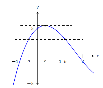
FIgure \(\PageIndex{2}\): A graph of \(f(x) = x^3-5x^2+3x+5\), where \(f(a) = f(b)\). Note the existence of \(c\), where \(a<c<b\), where \(f'(c)=0\).

Rolle's Theorem is really just a special case of the Mean Value Theorem. If \(f(a) = f(b)\), then the average rate of change on \((a,b)\) is \(0\), and the theorem guarantees some \(c\) where \(f'(c)=0\). We will prove Rolle's Theorem, then use it to prove the Mean Value Theorem.

Proof of Rolle's Theorem

Let \(f\) be differentiable on \((a,b)\) where \(f(a)=f(b)\). We consider two cases.

Case 1: Consider the case when \(f\) is constant on \([a,b]\); that is, \(f(x) = f(a) = f(b)\) for all \(x\) in \([a,b]\). Then \(f'(x) = 0\) for all \(x\) in \([a,b]\), showing there is at least one value \(c\) in \((a,b)\) where \(f'(c)=0\).

Case 2: Now assume that \(f\) is not constant on \([a,b]\). The Extreme Value Theorem guarantees that \(f\) has a maximal and minimal value on \([a,b]\), found either at the endpoints or at a critical value in \((a,b)\). Since \(f(a)=f(b)\) and \(f\) is not constant, it is clear that the maximum and minimum cannot both be found at the endpoints. Assume, without loss of generality, that the maximum of \(f\) is not found at the endpoints. Therefore there is a \(c\) in \((a,b)\) such that \(f(c)\) is the maximum value of \(f\). By Theorem 3.1.2, \(c\) must be a critical number of \(f\); since \(f\) is differentiable, we have that \(f'(c) = 0\), completing the proof of the theorem.

\(\square\)

We can now prove the Mean Value Theorem.

Proof of the Mean Value Theorem

Define the function

$$g(x) = f(x) - \frac{f(b)-f(a)}{b-a}x.\]

We know \(g\) is differentiable on \((a,b)\) and continuous on \([a,b]\) since \(f\) is. We can show \(g(a)=g(b)\) (it is actually easier to show \(g(b)-g(a)=0\), which suffices). We can then apply Rolle's theorem to guarantee the existence of \(c \in (a,b)\) such that \(g'(c) = 0\). But note that

$$0= g'(c) = f'(c) - \frac{f(b)-f(a)}{b-a} \ ;\]

hence

$$f'(c) = \frac{f(b)-f(a)}{b-a},\]

which is what we sought to prove.

\(\square\)

Going back to the very beginning of the section, we see that the only assumption we would need about our distance function \(f(t)\) is that it be continuous and differentiable for \(t\) from 0 to 2 hours (both reasonable assumptions). By the Mean Value Theorem, we are guaranteed a time during the trip where our instantaneous speed is 50 mph. This fact is used in practice. Some law enforcement agencies monitor traffic speeds while in aircraft. They do not measure speed with radar, but rather by timing individual cars as they pass over lines painted on the highway whose distances apart are known. The officer is able to measure the average speed of a car between the painted lines; if that average speed is greater than the posted speed limit, the officer is assured that the driver exceeded the speed limit at some time.

Note that the Mean Value Theorem is an existence theorem. It states that a special value \(c\) exists, but it does not give any indication about how to find it. It turns out that when we need the Mean Value Theorem, existence is all we need

Example \(\PageIndex{2}\): Using the Mean Value Theorem

Consider \(f(x) = x^3+5x+5\) on \([-3,3]\). Find \(c\) in \([-3,3]\) that satisfies the Mean Value Theorem.

Solution

The average rate of change of \(f\) on \([-3,3]\) is:

\[\frac{f(3)-f(-3)}{3-(-3)} = \frac{84}{6} = 14.\]

We want to find \(c\) such that \(f'(c) = 14\). We find \(f'(x) = 3x^2+5\). We set this equal to 14 and solve for \(x\).

\[ \begin{align*} f'(x) &= 14 \\ 3x^2 +5 &= 14\\ x^2 &= 3\\ x &= \pm \sqrt{3} \approx \pm 1.732 \end{align*}\]

We have found 2 values \(c\) in \([-3,3]\) where the instantaneous rate of change is equal to the average rate of change; the Mean Value Theorem guaranteed at least one. In Figure \(\PageIndex{3}\) \(f\) is graphed with a dashed line representing the average rate of change; the lines tangent to \(f\) at \(x=\pm \sqrt{3}\) are also given. Note how these lines are parallel (i.e., have the same slope) as the dashed line.

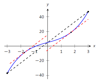
Figure \(\PageIndex{3}\): Demonstrating the Mean Value Theorem in Example \(\PageIndex{2}\).

While the Mean Value Theorem has practical use (for instance, the speed monitoring application mentioned before), it is mostly used to advance other theory. We will use it in the next section to relate the shape of a graph to its derivative.

Contributors and Attributions

• Gregory Hartman (Virginia Military Institute). Contributions were made by Troy Siemers and Dimplekumar Chalishajar of VMI and Brian Heinold of Mount Saint Mary's University. This content is copyrighted by a Creative Commons Attribution - Noncommercial (BY-NC) License. http://www.apexcalculus.com/

• Integrated by Justin Marshall.