7.1: Integration by Parts

Learning Objectives

• Recognize when to use integration by parts.
• Use the integration-by-parts formula to solve integration problems.
• Use the integration-by-parts formula for definite integrals.

By now we have a fairly thorough procedure for how to evaluate many basic integrals. However, although we can integrate $∫x \sin (x^2)\,dx$ by using the substitution, $u=x^2$, something as simple looking as $∫x\sin x\,\,dx$ defies us. Many students want to know whether there is a product rule for integration. There is not, but there is a technique based on the product rule for differentiation that allows us to exchange one integral for another. We call this technique integration by parts.

The Integration-by-Parts Formula

If, $h(x)=f(x)g(x)$, then by using the product rule, we obtain

$$h′(x)=f′(x)g(x)+g′(x)f(x). \label{eq1}$$

Although at first it may seem counterproductive, let’s now integrate both sides of Equation $\ref{eq1}$:

$$∫h′(x)\,\,dx=∫(g(x)f′(x)+f(x)g′(x))\,\,dx. \nonumber$$

This gives us

$$h(x)=f(x)g(x)=∫g(x)f′(x)\,dx+∫f(x)g′(x)\,\,dx. \nonumber$$

Now we solve for $∫f(x)g′(x)\,\,dx:$

$$∫f(x)g′(x)\,dx=f(x)g(x)−∫g(x)f′(x)\,\,dx. \nonumber$$

By making the substitutions $u=f(x)$ and $v=g(x)$, which in turn make $du=f′(x)\,dx$ and $dv=g′(x)\,dx$, we have the more compact form

$$∫u\,dv=uv−∫v\,du. \nonumber$$

Integration by Parts

Let $u=f(x)$ and $v=g(x)$ be functions with continuous derivatives. Then, the integration-by-parts formula for the integral involving these two functions is:

$$∫u\,dv=uv−∫v\,du. \label{IBP}$$

The advantage of using the integration-by-parts formula is that we can use it to exchange one integral for another, possibly easier, integral. The following example illustrates its use.

Example $\PageIndex{1}$: Using Integration by Parts

Use integration by parts with $u=x$ and $dv=\sin x\,\,dx$ to evaluate

$$∫x\sin x\,\,dx. \nonumber$$

Solution

By choosing $u=x$, we have $du=1\,\,dx$. Since $dv=\sin x\,\,dx$, we get

$$v=∫\sin x\,\,dx=−\cos x. \nonumber$$

It is handy to keep track of these values as follows:

• $u=x$
• $dv=\sin x\,\,dx$
• $du=1\,dx$
• $v=∫\sin x\,\,dx=−\cos x.$

Applying the integration-by-parts formula (Equation $\ref{IBP}$) results in

$$\begin{align} ∫x\sin x\,\,dx &=(x)(−\cos x)−∫(−\cos x)(1\,\,dx) \tag{Substitute} \\[4pt] &=−x\cos x+∫\cos x\,\,dx \tag{Simplify} \end{align}$$

Then use

$$∫\cos x\,\,dx =\sin x+C. \nonumber$$

to obtain

$$∫x\sin x\,\,dx =−x\cos x+\sin x+C. \nonumber$$

Analysis

At this point, there are probably a few items that need clarification. First of all, you may be curious about what would have happened if we had chosen $u=\sin x$ and $dv=x \, dx$. If we had done so, then we would have $du=\cos x$ and $v=\dfrac{1}{2}x^2$. Thus, after applying integration by parts (Equation $\ref{IBP}$), we have

$$∫​x\sin x\,\,dx=\dfrac{1}{2}x^2\sin x−∫\dfrac{1}{2}x^2\cos x\,\,dx. \nonumber$$

Unfortunately, with the new integral, we are in no better position than before. It is important to keep in mind that when we apply integration by parts, we may need to try several choices for $u$ and $dv$ before finding a choice that works.

Second, you may wonder why, when we find $v=∫​\sin x\,\,dx=−\cos x$, we do not use $v=−\cos x+K.$ To see that it makes no difference, we can rework the problem using $v=−\cos x+K$:

$$\begin{align*} ∫x\sin x\,\,dx &=(x)(−\cos x+K)−∫(−\cos x+K)(1\,\,dx) \\[4pt] &=−x\cos x+Kx+∫\cos x\,\,dx−∫K\,\,dx \\[4pt] &=−x\cos x+Kx+\sin x−Kx+C \\[4pt] &=−x\cos x+\sin x+C. \end{align*}$$

As you can see, it makes no difference in the final solution.

Last, we can check to make sure that our antiderivative is correct by differentiating $−x\cos x+\sin x+C:$

$$\begin{align*} \dfrac{d}{\,dx}(−x\cos x+\sin x+C) = \cancel{(−1)\cos x} + (−x)(−\sin x) + \cancel{\cos x} \\[4pt] =x\sin x \end{align*}$$

Therefore, the antiderivative checks out.

Exercise $\PageIndex{1}$

Evaluate $∫​xe^{2x}\,dx$ using the integration-by-parts formula (Equation $\ref{IBP}$) with $u=x$ and $dv=e^{2x}\,\,dx$.

Hint

Find $du$ and $v$, and use the previous example as a guide.

Answer

$$∫​xe^{2x}\,\,dx=\dfrac{1}{2}xe^{2x}−\dfrac{1}{4}e^{2x}+C \nonumber$$

The natural question to ask at this point is: How do we know how to choose $u$ and $dv$? Sometimes it is a matter of trial and error; however, the acronym LIATE can often help to take some of the guesswork out of our choices. This acronym stands for Logarithmic Functions, Inverse Trigonometric Functions, Algebraic Functions, Trigonometric Functions, and Exponential Functions. This mnemonic serves as an aid in determining an appropriate choice for $u$. The type of function in the integral that appears first in the list should be our first choice of $u$.

For example, if an integral contains a logarithmic function and an algebraic function, we should choose $u$ to be the logarithmic function, because L comes before A in LIATE. The integral in Example $\PageIndex{1}$ has a trigonometric function ($\sin x$) and an algebraic function ($x$). Because A comes before T in LIATE, we chose $u$ to be the algebraic function. When we have chosen $u$, $dv$ is selected to be the remaining part of the function to be integrated, together with $\,dx$.

Why does this mnemonic work? Remember that whatever we pick to be $dv$ must be something we can integrate. Since we do not have integration formulas that allow us to integrate simple logarithmic functions and inverse trigonometric functions, it makes sense that they should not be chosen as values for $dv$. Consequently, they should be at the head of the list as choices for $u$. Thus, we put LI at the beginning of the mnemonic. (We could just as easily have started with IL, since these two types of functions won’t appear together in an integration-by-parts problem.) The exponential and trigonometric functions are at the end of our list because they are fairly easy to integrate and make good choices for $dv$. Thus, we have TE at the end of our mnemonic. (We could just as easily have used ET at the end, since when these types of functions appear together it usually doesn’t really matter which one is $u$ and which one is $dv$.) Algebraic functions are generally easy both to integrate and to differentiate, and they come in the middle of the mnemonic.

Example $\PageIndex{2}$: Using Integration by Parts

Evaluate $$∫\dfrac{\ln x}{x^3}\,\,dx. \nonumber$$

Solution

Begin by rewriting the integral:

$$∫\dfrac{\ln x}{x^3}\,\,dx=∫​x^{−3}\ln x\,\,dx. \nonumber$$

Since this integral contains the algebraic function $x^{−3}$ and the logarithmic function $\ln x$, choose $u=\ln x$, since $L$ comes before A in LIATE. After we have chosen $u=\ln x$, we must choose $dv=x^{−3}\,dx$.

Next, since $u=\ln x,$ we have $du=\dfrac{1}{x}\,dx.$ Also, $v=∫​x^{−3}\,dx=−\dfrac{1}{2}x^{−2}.$ Summarizing,

• $u=\ln x$
• $du=\dfrac{1}{x}\,dx$
• $dv=x^{−3}\,dx$
• $v=∫​x^{−3}\,dx=−\dfrac{1}{2}x^{−2}.$

Substituting into the integration-by-parts formula (Equation $\ref{IBP}$) gives

$$\begin{align*} ∫\dfrac{\ln x}{x^3}\,dx &=∫​x^{−3}\ln x\,dx=(\ln x)(−\dfrac{1}{2}x^{−2})−∫​(−\dfrac{1}{2}x^{−2})(\dfrac{1}{x}\,dx) \\[4pt] &=−\dfrac{1}{2}x^{−2}\ln x+∫\dfrac{1}{2}x^{−3}\,\,dx \\[4pt] &=−\dfrac{1}{2}x^{−2}\ln x−\dfrac{1}{4}x^{−2}+C\ \\[4pt] &=−\dfrac{1}{2x^2}\ln x−\dfrac{1}{4x^2}+C \end{align*} \nonumber$$

Exercise $\PageIndex{2}$

Evaluate $$∫​x\ln x \,\,dx. \nonumber$$

Hint

Use $u=\ln x$ and $dv=x\,\,dx$.

Answer

$$∫​x\ln x \,\,dx=\dfrac{1}{2}x^2\ln x−\dfrac{1}{4}x^2+C \nonumber$$

In some cases, as in the next two examples, it may be necessary to apply integration by parts more than once.

Example $\PageIndex{3A}$: Applying Integration by Parts More Than Once

Evaluate $$∫​x^2e^{3x}\,dx. \nonumber$$

Solution

Using LIATE, choose $u=x^2$ and $dv=e^{3x}\,dx$. Thus, $du=2x\,dx$ and $v=∫e^{3x}\,dx=\left(\dfrac{1}{3}\right)e^{3x}$. Therefore,

• $u=x^2$
• $du=2x\,dx$
• $dv=e^{3x}\,dx$
• $v=∫e^{3x}\,dx=\dfrac{1}{3}e^{3x}.$

Substituting into Equation $\ref{IBP}$ produces

$$∫x^2e^{3x}\,dx=\dfrac{1}{3}x^2e^{3x}−∫\dfrac{2}{3}xe^{3x}\,dx. \label{3A.2}$$

We still cannot integrate $∫\dfrac{2}{3}xe^{3x}\,dx$ directly, but the integral now has a lower power on $x$. We can evaluate this new integral by using integration by parts again. To do this, choose

$$u=x \nonumber$$

and

$$dv=\dfrac{2}{3}e^{3x}\,dx. \nonumber$$

Thus,

$$du=\,dx \nonumber$$

and

$$v=∫\left(\dfrac{2}{3}\right)e^{3x}\,dx=\left(\dfrac{2}{9}\right)e^{3x}. \nonumber$$

Now we have

• $u=x$
• $du=\,dx$
• $dv=\dfrac{2}{3}e^{3x}\,dx$
• $\displaystyle v=∫\dfrac{2}{3}e^{3x}\,dx=\dfrac{2}{9}e^{3x}.$

Substituting back into Equation $\ref{3A.2}$ yields

$$∫​x^2e^{3x}\,dx=\dfrac{1}{3}x^2e^{3x}−\left(\dfrac{2}{9}xe^{3x}−∫\dfrac{​2}{9}e^{3x}\,dx\right). \nonumber$$

After evaluating the last integral and simplifying, we obtain

$$∫x^2e^{3x}\,dx=\dfrac{1}{3}x^2e^{3x}−\dfrac{2}{9}xe^{3x}+\dfrac{2}{27}e^{3x}+C. \nonumber$$

Example $\PageIndex{3B}$: Applying Integration by Parts When LIATE Does not Quite Work

Evaluate

$$∫​t^3e^{t^2}dt. \nonumber$$

Solution

If we use a strict interpretation of the mnemonic LIATE to make our choice of $u$, we end up with $u=t^3$ and $dv=e^{t^2}dt$. Unfortunately, this choice won’t work because we are unable to evaluate $∫​e^{t^2}dt$. However, since we can evaluate $∫​te^{t^2}\,dx$, we can try choosing $u=t^2$ and $dv=te^{t^2}dt.$ With these choices we have

• $u=t^2$
• $du=2tdt$
• $dv=te^{t^2}dt$
• $v=∫​te^{t^2}dt=\dfrac{1}{2}e^{t^2}.$

Thus, we obtain

$$\begin{align*} ∫t^3e^{t^2}dt =\dfrac{1}{2}t^2e^{t^2}−∫\dfrac{1}{2}e^{t^2}2t\,dt \\[4pt] =\dfrac{1}{2}t^2e^{t^2}−\dfrac{1}{2}e^{t^2}+C. \end{align*}$$

Example $\PageIndex{3C}$: Applying Integration by Parts More Than Once

Evaluate $$∫​\sin (\ln x)\,dx. \nonumber$$

Solution

This integral appears to have only one function—namely, $\sin (\ln x)$—however, we can always use the constant function 1 as the other function. In this example, let’s choose $u=\sin (\ln x)$ and $dv=1\,dx$. (The decision to use $u=\sin (\ln x)$ is easy. We can’t choose $dv=\sin (\ln x)\,dx$ because if we could integrate it, we wouldn’t be using integration by parts in the first place!) Consequently, $du=(1/x)\cos (\ln x) \,dx$ and $v=∫​ 1 \,dx=x.$ After applying integration by parts to the integral and simplifying, we have

$$∫​\sin \left(\ln x\right) \,dx=x \sin (\ln x)−\int \cos (\ln x)\,dx. \nonumber$$

Unfortunately, this process leaves us with a new integral that is very similar to the original. However, let’s see what happens when we apply integration by parts again. This time let’s choose $u=\cos (\ln x)$ and $dv=1\,dx,$ making $du=−(1/x)\sin (\ln x)\,dx$ and $v=∫​1\,dx=x.$

Substituting, we have

$$∫​\sin (\ln x)\,dx=x \sin (\ln x)−(x \cos (\ln x)-∫​−\sin (\ln x)\,dx). \nonumber$$

After simplifying, we obtain

$$∫​\sin (\ln x)\,dx=x\sin (\ln x)−x \cos (\ln x)−∫​\sin (\ln x)\,dx. \nonumber$$

The last integral is now the same as the original. It may seem that we have simply gone in a circle, but now we can actually evaluate the integral. To see how to do this more clearly, substitute $I=∫​\sin (\ln x)\,dx.$ Thus, the equation becomes

$$I=x \sin (\ln x)−x \cos (\ln x)−I. \nonumber$$

First, add $I$ to both sides of the equation to obtain

$$2I=x \sin (\ln x)−x \cos (\ln x). \nonumber$$

Next, divide by 2:

$$I=\dfrac{1}{2}x \sin (\ln x)−\dfrac{1}{2}x \cos (\ln x). \nonumber$$

Substituting $I=∫​\sin (\ln x)\,dx$ again, we have

$$\int \sin (\ln x) \,dx=\dfrac{1}{2}x \sin (\ln x)−\dfrac{1}{2}x \cos (\ln x). \nonumber$$

From this we see that $(1/2)x \sin (\ln x)−(1/2)x \cos (\ln x)$ is an antiderivative of $\sin (\ln x)\,dx$. For the most general antiderivative, add $+C$:

$$∫ \sin (\ln x) \,dx=\dfrac{1}{2}x \sin (\ln x)−\dfrac{1}{2}x \cos (\ln x)+C. \nonumber$$

Analysis

If this method feels a little strange at first, we can check the answer by differentiation:

$$\begin{align*} \dfrac{d}{\,dx}\left(\dfrac{1}{2}x \sin (\ln x)−\dfrac{1}{2}x\cos (\ln x)\right) \\[4pt] &=\dfrac{1}{2}(\sin (\ln x))+\cos (\ln x)⋅\dfrac{1}{x}⋅\dfrac{1}{2}x−\left(\dfrac{1}{2}\cos (\ln x)−\sin (\ln x)⋅\dfrac{1}{x}⋅\dfrac{1}{2}x\right) \\[4pt] &=\sin (\ln x). \end{align*}$$

Exercise $\PageIndex{3}$

Evaluate $$∫x^2\sin x\,dx. \nonumber$$

Hint

This is similar to Examples $\PageIndex{3A}$ - $\PageIndex{3C}$.

Answer

$$∫x^2\sin x\,dx=−x^2\cos x+2x\sin x+2\cos x+C \nonumber$$

Integration by Parts for Definite Integrals

Now that we have used integration by parts successfully to evaluate indefinite integrals, we turn our attention to definite integrals. The integration technique is really the same, only we add a step to evaluate the integral at the upper and lower limits of integration.

Integration by Parts for Definite Integrals

Let $u=f(x)$ and $v=g(x)$ be functions with continuous derivatives on [$a,b$]. Then

$$∫^b_a u\,dv=uv\Big|^b_a−∫^b_a v\, du \nonumber$$

Example $\PageIndex{4A}$: Finding the Area of a Region

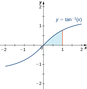
Find the area of the region bounded above by the graph of $y=\tan^{−1}x$ and below by the $x$-axis over the interval [$0,1$].

Solution

This region is shown in Figure $\PageIndex{1}$. To find the area, we must evaluate

$$∫^1_0 \tan^{−1}x\, \,dx. \nonumber$$

Figure $\PageIndex{1}$: To find the area of the shaded region, we have to use integration by parts.

For this integral, let’s choose $u=tan^{−1}x$ and $dv=\,dx$, thereby making $du=\dfrac{1}{x^2+1}\,dx$ and $v=x$. After applying the integration-by-parts formula (Equation $\ref{IBP}$) we obtain

$$\text{Area}=\left. x \tan^{−1} x \right|^1_0−∫^1_0 \dfrac{x}{x^2+1} \,dx. \nonumber$$

Use $u$-substitution to obtain

$$∫^1_0\dfrac{x}{x^2+1}\,dx=\left.\dfrac{1}{2}\ln \left(x^2+1\right) \right|^1_0. \nonumber$$

Thus,

$$\text{Area}=x \tan^{−1}x \Big|^1_0− \left.\dfrac{1}{2}\ln \left( x^2+1 \right) \right|^1_0=\left(\dfrac{π}{4}−\dfrac{1}{2}\ln 2\right) \,\text{units}^2. \nonumber$$

At this point it might not be a bad idea to do a “reality check” on the reasonableness of our solution. Since $\dfrac{π}{4}−\dfrac{1}{2}\ln 2≈0.4388\,\text{units}^2,$ and from Figure $\PageIndex{1}$ we expect our area to be slightly less than $0.5\,\text{units}^2,$ this solution appears to be reasonable.

Example $\PageIndex{4B}$: Finding a Volume of Revolution

Find the volume of the solid obtained by revolving the region bounded by the graph of $f(x)=e^{−x},$ the $x$-axis, the $y$-axis, and the line $x=1$ about the $y$-axis.

Solution

The best option to solving this problem is to use the shell method. Begin by sketching the region to be revolved, along with a typical rectangle (Figure $\PageIndex{2}$).

Figure $\PageIndex{2}$: We can use the shell method to find a volume of revolution.

To find the volume using shells, we must evaluate

$$2π∫^1_0xe^{−x}\,dx. \label{4B.1}$$

To do this, let $u=x$ and $dv=e^{−x}$. These choices lead to $du=\,dx$ and $v=∫​e^{−x}\,dx=−e^{−x}.$ Using the Shell Method formula, we obtain

$$\begin{align*} \text{Volume} &=2π∫^1_0xe^{−x}\,dx \\[4pt] = 2π\left(−xe^{−x}\Big|^1_0+∫^1_0e^{−x}\,dx \right) \tag{Use integration by parts} \\[4pt] &= 2π\left( -e^{-1} + 0 - e^{-x}\Big|^1_0\right) \\[4pt] &= 2π\left( -e^{-1} - e^{-1} + 1 \right) \\[4pt] &= 2π\left(1 - \dfrac{2}{e}\right)\,\text{units}^3.\tag{Evaluate and simplify} \end{align*}$$

Analysis

Again, it is a good idea to check the reasonableness of our solution. We observe that the solid has a volume slightly less than that of a cylinder of radius $1$ and height of $1/e$ added to the volume of a cone of base radius $1$ and height of $1−\dfrac{1}{e}.$ Consequently, the solid should have a volume a bit less than

$$π(1)^2\dfrac{1}{e}+\left(\dfrac{π}{3}\right)(1)^2\left(1−\dfrac{1}{e}\right)=\dfrac{2π}{3e}+\dfrac{π}{3}≈1.8177\,\text{units}^3. \nonumber$$

Since $2π−\dfrac{4π}{e}≈1.6603,$ we see that our calculated volume is reasonable.

Exercise $\PageIndex{4}$

Evaluate $$∫^{π/2}_0x\cos x\,dx. \nonumber$$

Hint

Use Equation $\ref{IBP}$ with $u=x$ and $dv=\cos x\,dx.$

Answer

$$∫^{π/2}_0x\cos x\,dx = \dfrac{π}{2}−1 \nonumber$$

Key Concepts

• The integration-by-parts formula (Equation $\ref{IBP}$) allows the exchange of one integral for another, possibly easier, integral.
• Integration by parts applies to both definite and indefinite integrals.

Key Equations

• Integration by parts formula

$\displaystyle ∫u\,dv=uv−∫v\,du$

• Integration by parts for definite integrals

$\displaystyle ∫^b_au\,dv=uv\Big|^b_a−∫^b_av\,du$

Glossary

integration by parts

a technique of integration that allows the exchange of one integral for another using the formula $\displaystyle ∫​u\,dv=uv−∫​v\,du$