6.5: Bayes' Formula

Learning Objectives

In this section, you will learn to:

• Find probabilities using Bayes’ formula.
• Use a probability tree to find and represent values needed when using Bayes’ formula.

Prerequisite Skills

Before you get started, take this prerequisite quiz.

1. If \(P(F) = .4\), \(P(E | F) = .3\), find \(P\)(\(E \cap F\)).

Click here to check your answer

\(.12\)

If you missed this problem, review Section 6.4. (Note that this will open in a new window.)

 

2. \(P(E) = .3\), \(P(F) = .3\); \(E \cap F\) are mutually exclusive. Find \(P(E | F)\).

Click here to check your answer

\(.3\)

If you missed this problem, review Section 6.4. (Note that this will open in a new window.)

 

3. If \(P(E) = .6\), \(P\)(\(E \cap F\)) = .24, find \(P(F | E)\).

Click here to check your answer

\(.4\)

If you missed this problem, review Section 6.4. (Note that this will open in a new window.)

 

4. If \(P(E \cap F\)) = \(.04\) , \(P(E | F) = .1\), find \(P(F)\).

Click here to check your answer

\(.4\)

If you missed this problem, review Section 6.4. (Note that this will open in a new window.)

In this section, we will develop and use Bayes' Formula to solve an important type of probability problem. Bayes' formula is a method of calculating the conditional probability \(P(F | E)\) from \(P(E | F)\). The ideas involved here are not new, and most of these problems can be solved using a tree diagram. However, Bayes' formula does provide us with a tool with which we can solve these problems without a tree diagram.

We begin with an example.

Example \(\PageIndex{1}\)

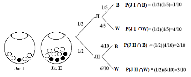
Suppose you are given two jars. Jar I contains one black and 4 white marbles, and Jar II contains 4 black and 6 white marbles. A jar and a marble are selected at random.  Construct a tree diagram to represent this scenario and to answer the following questions.

1. What is the probability that the marble chosen is a black marble?
2. If the chosen marble is black, what is the probability that it came from Jar I?
3. If the chosen marble is black, what is the probability that it came from Jar II?

Solution

Let \(J I\) be the event that Jar I is chosen, \(J II\) be the event that Jar II is chosen, \(B\) be the event that a black marble is chosen and \(W\) the event that a white marble is chosen.

We illustrate using a tree diagram.

1. The probability that a black marble is chosen is \(P(B)\) = 1/10 + 2/10 = 3/10.
2. To find \(P(J I | B)\), we use the definition of conditional probability, and we get \[P(J I | B)=\frac{P(J I \cap B)}{P(B)}=\frac{1 / 10}{3 / 10}=\frac{1}{3} \nonumber\]
3. Similarly, \(\mathrm{P}(\mathrm{J} \mathrm{II} | \mathrm{B})=\frac{\mathrm{P}(\mathrm{J} \mathrm{II} \cap \mathrm{B})}{\mathrm{P}(\mathrm{B})}=\frac{2 / 10}{3 / 10}=\frac{2}{3}\)

In parts b and c, the reader should note that the denominator is the sum of all probabilities of all branches of the tree that produce a black marble, while the numerator is the branch that is associated with the particular jar in question.

We will soon discover that this is a statement of Bayes' formula.

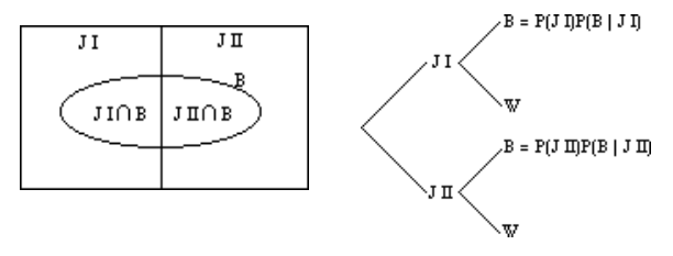
Let us first visualize the problem.

We are given a sample space \(\mathrm{S}\) and two mutually exclusive events \(J I\) and \(J II\). That is, the two events, \(J I\) and \(J II\), divide the sample space into two parts such that \(\mathrm{JI} \cup \mathrm{JII}=\mathrm{S}\). Furthermore, we are given an event \(B\) that has elements in both \(J I\) and \(J II\), as shown in the Venn diagram below.

From the Venn diagram, we can see that \(\mathrm{B}=(\mathrm{B} \cap \mathrm{J} \mathrm{I}) \cup(\mathrm{B} \cap \mathrm{J} \mathrm{II})\) Therefore:

\[ P(B)=P(B \cap J I)+P(B \cap J I I) \nonumber \]

But the multiplication rule in Section 6.5 gives us

\[ P(B \cap J I)=P(J I) \cdot P(B | J I) \quad \text { and } \quad P(B \cap J I I)=P(J I I) \cdot P(B | J I I) \nonumber\]

By substitution, we get

\[P(B)=P(J I) \cdot P(B | J I)+P(J I I) \cdot P(B | J I I) \nonumber\]

The conditional probability formula gives us

\[P(J I | B)=\frac{P(J I \cap B)}{P(B)} \nonumber\]

Therefore, \(P(J I | B)=\frac{P(J I) \cdot P(B | J I)}{P(B)}\)

or

\[P(J I | B)=\frac{P(J I) \cdot P(B | J I)}{P(J I) \cdot P(B | J I)+P(J I I) \cdot P(B | J I I)} \nonumber\]

The last statement is Bayes' Formula for the case where the sample space is divided into two partitions.

The following is the generalization of Bayes’ formula for n partitions.

Bayes' Formula for \(n\) partitions

Let \(\mathrm{S}\) be a sample space that is divided into \(n\) partitions, \(A_1\), \(A_2\), . . . \(A_n\). If \(E\) is any event in \(\mathrm{S}\), then

\[\mathbf{P}\left(\mathbf{A}_{\mathbf{i}} | \mathbf{E}\right)=\frac{\mathbf{P}\left(\mathbf{E} | \mathbf{A}_{\mathbf{i}}\right)\mathbf{P}\left(\mathbf{A}_{\mathbf{i}}\right)}{\mathbf{P}\left(\mathbf{E} | \mathbf{A}_{\mathbf{1}}\right)\mathbf{P}\left(\mathbf{A}_{\mathbf{1}}\right) +\mathbf{P}\left(\mathbf{E} | \mathbf{A}_{2}\right)\mathbf{P}\left(\mathbf{A}_{2}\right) +\cdots+\mathbf{P}\left(\mathbf{E} | \mathbf{A}_{\mathbf{n}}\right)\mathbf{P}\left(\mathbf{A}_{\mathbf{n}}\right) } \nonumber\]

Note that this can be summarized as \[\mathbf{P}\left(\mathbf{A}_{\mathbf{i}} | \mathbf{E}\right)=\frac{\text{product of branches leading to E through } \mathbf{A}_{\mathbf{i}}}{\text{sum of branch products leading to E}} \nonumber \]

We begin with the following example.

Example \(\PageIndex{2}\)

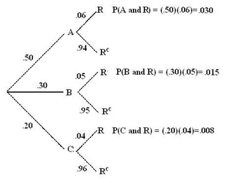
A department store buys 50% of its appliances from Manufacturer A, 30% from Manufacturer B, and 20% from Manufacturer C. It is estimated that 6% of Manufacturer A's appliances, 5% of Manufacturer B's appliances, and 4% of Manufacturer C's appliances need repair before the warranty expires. An appliance is chosen at random. If the appliance chosen needed repair before the warranty expired, what is the probability that the appliance was manufactured by Manufacturer A? Manufacturer B? Manufacturer C?

Solution

Let A, B and C be the events that the appliance is manufactured by Manufacturer A, Manufacturer B, and Manufacturer C, respectively. Further, suppose that the event R denotes that the appliance needs repair before the warranty expires.

We need to find P(A | R), P(B | R) and P(C | R).

We will do this problem both by using a tree diagram and by using Bayes' formula.

We draw a tree diagram.

The probability P(A | R), for example, is a fraction whose denominator is the sum of all probabilities of all branches of the tree that result in an appliance that needs repair before the warranty expires, and the numerator is the branch that is associated with Manufacturer A. P(B | R) and P(C | R) are found in the same way.

\[\begin{array}{l}
P(A | R)=\frac{.030}{(.030)+(.015)+(.008)}=\frac{.030}{.053}=.566 \\
P(B | R)=\frac{.015}{.053}=.283 \text { and } P(C | R)=\frac{.008}{.053}=.151
\end{array} \nonumber\]

Alternatively, using Bayes' formula,

\begin{aligned}
\mathrm{P}(\mathrm{A} | \mathrm{R}) &=\frac{\mathrm{P}(\mathrm{R} | \mathrm{A})\mathrm{P}(\mathrm{A}) }{\mathrm{P}(\mathrm{R} | \mathrm{A})\mathrm{P}(\mathrm{A}) + \mathrm{P}(\mathrm{R} | \mathrm{B})\mathrm{P}(\mathrm{B}) + \mathrm{P}(\mathrm{R} | \mathrm{C})\mathrm{P}(\mathrm{C}) } \\
&=\frac{.030}{(.030)+(.015)+(.008)}=\frac{.030}{.053}=.566
\end{aligned}

P(B | R) and P(C | R) can be determined in the same manner.

P(B | R) = \(\frac{.015}{.053}=.283\) and P(C | R) = \(\frac{.008}{.053}=.151\).

Example \(\PageIndex{3}\)

There are five American Furniture Warehouse stores in the Denver area. The percent of employees over the age of 50 is given in the table below.

Store Number	Number of Employees	Percent of 50+ Employees
1	300	.40
2	150	.65
3	200	.60
4	250	.50
5	100	.70
	Total = 1000

If an employee chosen at random is over 50 years old, what is the probability that the employee works at store III?

Solution

Let \(k\) = 1, 2, . . . , 5 be the event that the employee worked at store \(k\), and A be the event that the employee is over 50 years old. Since there are a total of 1000 employees at the five stores,

\[P(1)=.30 \quad P(2)=.15 \quad P(3)=.20 \quad P(4)=.25 \quad P(5)=.10 \nonumber\]

Using Bayes' formula,

\[\begin{array}{l}
\mathrm{P}(3 | \mathrm{A})&=\frac{\mathrm{P}(\mathrm{A} | 3)\mathrm{P}(3) }{\mathrm{P}(\mathrm{A} | 1)\mathrm{P}(1) + \mathrm{P}(\mathrm{A} | 2)\mathrm{P}(2) + \mathrm{P}(\mathrm{A} | 3)\mathrm{P}(3) + \mathrm{P}(\mathrm{A} | 4)\mathrm{P}(4) + \mathrm{P}(\mathrm{A} | 5)\mathrm{P}(5) } \\
&=\frac{(.60)(.20)}{(.40)(.30)+(.65)(.15)+(.60)(.20)+(.50)(.25)+(.70)(.10)} \\
&=.2254
\end{array} \nonumber\]