
12.5: Acceleration and Kepler's Laws


- Last updated
- Jan 6, 2020
- Save as PDF
( \newcommand{\kernel}{\mathrm{null}\,}\)
Components of the Acceleration Vector
We can combine some of the concepts discussed in Arc Length and Curvature with the acceleration vector to gain a deeper understanding of how this vector relates to motion in the plane and in space. Recall that the unit tangent vector ⇀T and the unit normal vector ⇀N form an osculating plane at any point P on the curve defined by a vector-valued function ⇀r(t). The following theorem shows that the acceleration vector ⇀a(t) lies in the osculating plane and can be written as a linear combination of the unit tangent and the unit normal vectors.
Theorem 12.5.1: The Plane of the Acceleration Vector
The acceleration vector ⇀a(t) of an object moving along a curve traced out by a twice-differentiable function ⇀r(t) lies in the plane formed by the unit tangent vector ⇀T(t) and the principal unit normal vector ⇀N(t) to C.
Furthermore,
⇀a(t)=v′(t)⇀T(t)+[v(t)]2κ⇀N(t)
Here, v(t)=‖⇀v(t)‖ is the speed of the object and κ is the curvature of C traced out by ⇀r(t).
Proof
Because ⇀v(t)=⇀r′(t) and ⇀T(t)=⇀r′(t)||⇀r′(t)||, we have ⇀v(t)=||⇀r′(t)||⇀T(t)=v(t)⇀T(t).
Now we differentiate this equation:
⇀a(t)=⇀v′(t)=ddt(v(t)⇀T(t))=v′(t)⇀T(t)+v(t)⇀T′(t)
Since ⇀N(t)=⇀T′(t)||⇀T′(t)||, we know ⇀T′(t)=||⇀T′(t)||⇀N(t), so
⇀a(t)=v′(t)⇀T(t)+v(t)||⇀T′(t)||⇀N(t).
A formula for curvature is κ=||⇀T′(t)||||⇀r′(t)||, so ⇀T′(t)=κ||⇀r′(t)||=κv(t).
This gives ⇀a(t)=v′(t)⇀T(t)+κ(v(t))2⇀N(t).
◻
The real-valued coefficients of ⇀T(t) and ⇀N(t) (possibly real-valued functions of t) are referred to as the tangential component of acceleration and the normal component of acceleration, respectively. We write a⇀T to denote the tangential component and a⇀N to denote the normal component. Note that these names are a little misleading, as these functions of t are not vector components, but the magnitudes of the corresponding vector components of acceleration.
Theorem 12.5.2: Tangential and Normal Components of Acceleration (as scalar magnitudes)
Let ⇀r(t) be a vector-valued function that denotes the position of an object as a function of time. Then ⇀a(t)=⇀r′′(t) is the acceleration vector. The tangential and normal components of acceleration a⇀T and a⇀N (the magnitudes of the corresponding vector components of acceleration) are given by the formulas
a⇀T=⇀a⋅⇀T=⇀v⋅⇀a||⇀v||
and
a⇀N=⇀a⋅⇀N=||⇀v×⇀a||||⇀v||=√||⇀a||2−(a⇀T)2.
The vector components of acceleration are related by the formula
⇀a(t)=a⇀T⇀T(t)+a⇀N⇀N(t).
Here ⇀T(t) is the unit tangent vector to the curve defined by ⇀r(t), and ⇀N(t) is the unit normal vector to the curve defined by ⇀r(t).
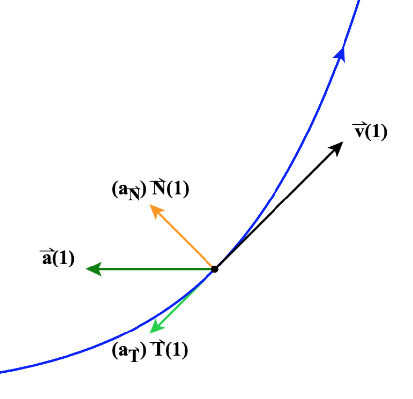
Figure 12.5.1: The acceleration can be broken into components parallel to ⇀N(t) and ⇀T(t). Here t=1.
At a given point on the curve, breaking the acceleration vector up into these two components, a tangential component parallel to the velocity vector (and ⇀T) and a normal component parallel to the normal vector ⇀N, allows us to more clearly see the effect of the acceleration vector on the velocity at that point. See Figure 12.5.1.
Only the component of acceleration that is parallel to the velocity will change the speed of the motion (affecting the magnitude of the velocity). And only the component that is normal to the curve will affect the direction of the velocity (and the corresponding bending of the curve at this point). Note that for the example in Figure 12.5.1, the acceleration is clearly slowing the velocity and turning the curve to the left.
This means that if acceleration is orthogonal to the velocity, it will only affect the direction and will not change the speed at this point. And if the acceleration is parallel to the velocity, it will only affect the speed and not change the direction at this point. If the acceleration vector is always parallel to the velocity vector for a given position function, the motion must be along a straight line.
Exercise 12.5.1
What can you say about the speed of the motion along a curve if the acceleration vector is always orthogonal to the velocity vector for the corresponding position function?
- Hint
-
In addition to considering what this means based on the discussion of the components of acceleration shown above, see Derivative Property vii in Section 12.2, considering what it says should be true if ⇀r′(t)⋅⇀r″(t)=0, that is, if ⇀v(t)⋅⇀a(t)=0.
Note that in this context, the unit vectors ⇀T(t) and ⇀N(t) are filling a role very similar to ˆi and ˆj. But instead of representing a vector in the xy-plane where the vectors ˆi and ˆj reside, the linear combination of ⇀T(t) and ⇀N(t) represents an acceleration vector in the plane formed by the vectors ⇀T(t) and ⇀N(t).
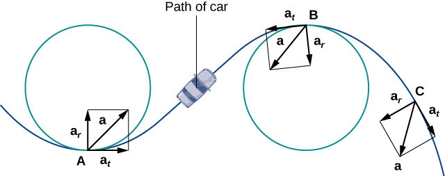
The normal component of acceleration is also called the centripetal component of acceleration or sometimes the radial component of acceleration. To understand centripetal acceleration, suppose you are traveling in a car on a circular track at a constant speed. Then, as we saw earlier, the acceleration vector points toward the center of the track at all times. As a rider in the car, you feel a pull toward the outside of the track because you are constantly turning. This sensation acts in the opposite direction of centripetal acceleration. The same holds true for non-circular paths. The reason is that your body tends to travel in a straight line and resists the force resulting from acceleration that push it toward the side. Note that at point B in Figure 12.5.2 the acceleration vector is pointing backward. This is because the car is decelerating as it goes into the curve.
The tangential and normal unit vectors at any given point on the curve provide a frame of reference at that point. The tangential and normal components of acceleration (as vectors) are the projections of the acceleration vector onto ⇀T and ⇀N, respectively.
Note that there are two ways for us to calculate the vector components of acceleration that are tangent and normal to the curve. We can either use the formulas in Theorem 12.5.2 above and multiply them by the unit tangent vector and the unit normal vector, respectively, or we can calculate these vectors directly (with a lot less effort) as the projection of the acceleration vector onto the velocity vector and the corresponding component of acceleration that is perpendicular to the velocity vector and that together with the projection sums to the original acceleration vector. We can thus use the simpler approach shown in Theorem 12.5.3 below.
Let ⇀r(t) be a vector-valued function that denotes the position of an object as a function of time. Then ⇀a(t)=⇀r′′(t) is the acceleration vector. The tangential and normal components of acceleration a⇀T⇀T(t) and a⇀N⇀N(t) are given by the formulas
a⇀T⇀T(t)=Proj⇀v(t)⇀a(t)The vector component of acceleration tangent to the curve
and
a⇀N⇀N(t)=⇀a(t)perp=⇀a(t)−Proj⇀v(t)⇀a(t)The vector component of acceleration normal to the curve
If we have already calculated ⇀T(t) and ⇀N(t), we can also determine these vector components of acceleration using these and the values of a⇀T and a⇀N from above.
Example 12.5.1: Finding Components of Acceleration (as magnitudes)
A particle moves in a path defined by the vector-valued function ⇀r(t)=t2ˆi+(2t−3)ˆj+(3t2−3t)ˆk, where t measures time in seconds and distance is measured in feet.
- Find a⇀T and a⇀N as functions of t.
- Find a⇀T and a⇀N at time t=2.
Solution
- Let’s start deriving the velocity and acceleration functions
⇀v(t)=⇀r′(t)=2tˆi+2ˆj+(6t−3)ˆk
⇀a(t)=⇀v′(t)=2ˆi+6ˆk
Now we use Equation ???:
a⇀T=⇀v⋅⇀a||⇀v||=(2tˆi+2ˆj+(6t−3)ˆk)⋅(2ˆi+6ˆk)||2tˆi+2ˆj+(6t−3)ˆk||=4t+6(6t−3)√(2t)2+22+(6t−3)2=40t−1840t2−36t+13
Then we apply Equation ???:a⇀N=√||⇀a||2−(a⇀T)2=√||2ˆi+6ˆk||2−(40t−18√40t2−36t+13)2=√4+36−(40t−18)240t2−36t+13=√40(40t2−36t+13)−(1600t2−1440t+324)40t2−36t+13=√19640t2−36t+13=14√40t2−36t+13
- We must evaluate each of the answers from part a at t=2:
a⇀T(2)=40(2)−18√40(2)2−36(2)+13=80−18√160−72+13=62√101=62√101101a⇀N(2)=14√40(2)2−36(2)+13=14√160−72+13=14√101=14√101101.
The units of acceleration are feet per second squared, as are the units of the normal and tangential components of acceleration.
Exercise 12.5.2
An object moves in a path defined by the vector-valued function ⇀r(t)=4tˆi+t2ˆj, where t measures time in seconds.
- Find a⇀T and a⇀N as functions of t.
- Find a⇀T and a⇀N at time t=−3.
- Hint
-
Use Equations ??? and ???
- Answer
-
a. a⇀T=⇀v(t)⋅⇀a(t)||⇀v(t)||=⇀r′(t)⋅⇀r″(t)||⇀r′(t)||=(4ˆi+2tˆj)⋅(2ˆj)||4ˆi+2tˆj||=4t√42+(2t)2=2t√2+t2
a⇀N=√||⇀a||2−a2⇀T=√||2ˆj||2−(2t√2+t2)2=√4−4t22+t2b. a⇀T(−3)=2(−3)√2+(−3)2=−6√11
a⇀N(−3)=√4−4(−3)22+(−3)2=√4−3611=√811=2√2√11
Now let's calculate the vector components of acceleration for the vector-valued function in Example 12.5.1. We'll start by calculating these vector components at a time t=2 using the projection of the acceleration vector onto the velocity vector at that time. Then we'll show the same approach to finding the vector components of acceleration as functions of t.
A particle moves in a path defined by the vector-valued function ⇀r(t)=t2ˆi+(2t−3)ˆj+(3t2−3t)ˆk, where t measures time in seconds and distance is measured in feet.
- Find the vector components of acceleration at time t=2.
- Find the vector components of the acceleration tangent and normal to the curve as functions of t.
Solution
From our work above, we have
⇀v(t)=⇀r′(t)=2tˆi+2ˆj+(6t−3)ˆk
⇀a(t)=⇀v′(t)=2ˆi+6ˆk
a. At time t=2, we have
⇀v(2)=2(2)ˆi+2ˆj+(6(2)−3)ˆk=4ˆi+2ˆj+9ˆk
and
⇀a(2)=2ˆi+6ˆk
Then the component of acceleration tangent to the curve at time t=2 is:
a⇀T⇀T(2)=Proj⇀v(2)⇀a(2)=⇀a(2)⋅⇀v(2)‖⇀v(2)‖⏟a⇀T(2)⋅⇀v(2)‖⇀v(2)‖⏟⇀T(2)
Since ⇀a(2)⋅⇀v(2)=2(4)+0(2)+6(9)=8+0+54=62,
and ‖⇀v(2)‖=√42+22+92=√16+4+81=√101,
a⇀T⇀T(2)=Proj⇀v(2)⇀a(2)=⇀a(2)⋅⇀v(2)‖⇀v(2)‖⋅⇀v(2)‖⇀v(2)‖=62101⇀v(2)=248101ˆi+124101ˆj+558101ˆk
Since the sum of these two components is ⇀a(2), the component of acceleration normal to the curve at time t=2 is:
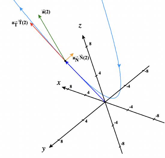
\begin{align*} a_\vecs{N}\vecs N(2) &= \vecs a(2)_{\text{perp}} = \vecs a(2) - \text{Proj}_{\vecs v(2)} \vecs a(2)\\[4pt] &= 2 \,\hat{\mathbf i} + 6 \,\hat{\mathbf k} - \left(\frac{248}{101} \,\hat{\mathbf i} +\frac{124}{101} \,\hat{\mathbf j} + \frac{558}{101} \,\hat{\mathbf k} \right) \\[4pt] &= \left(2 - \frac{248}{101}\right) \,\hat{\mathbf i} - \frac{124}{101} \,\hat{\mathbf j} + \left(6 - \frac{558}{101}\right) \,\hat{\mathbf k}\\[4pt] &= -\frac{46}{101} \,\hat{\mathbf i} - \frac{124}{101} \,\hat{\mathbf j} + \frac{48}{101} \,\hat{\mathbf k} \end{align*}
See the vector \vecs a(2) and its component vectors in Figure \PageIndex{3} below.
b. The more general vector components of acceleration (as functions of t) can be found in the same way with somewhat less work than taking time to first directly determine \vecs T(t) and \vecs N(t).
Since
\vecs{v}(t) = \vecs{r}'(t) = 2t\,\hat{\mathbf i}+2\,\hat{\mathbf j}+(6t-3)\,\hat{\mathbf k}\nonumber
and
\vecs{a}(t) = \vecs{v}'(t)=2\,\hat{\mathbf i}+6\,\hat{\mathbf k} \nonumber
we have
a_\vecs{T}\vecs T(t) = \text{Proj}_{\vecs v(t)} \vecs a(t) = \underbrace{\frac{\vecs a(t) \cdot \vecs v(t)}{\|\vecs v(t)\|}}_{a_{\vecs T}(t)}\cdot \underbrace{\frac{\vecs v(t)}{\|\vecs v(t)\|}}_{\vecs T(t)}\nonumber
As in part (a), we calculate \vecs a(t) \cdot \vecs v(t) = 2(2t) + 0(2) + 6(6t-3) = 4t + 0 + 36t - 18 = 40t - 18,
and \begin{align*} \|\vecs v(t)\| &= \sqrt{(2t)^2 + 2^2 + (6t-3)^2} \\[4pt] &= \sqrt{4t^2 + 4 + 36t^2 - 36t + 9} \\[4pt] &= \sqrt{40t^2 - 36t + 13}. \end{align*}
Then the vector component of acceleration tangent to the curve at time t is
\begin{align*} a_\vecs{T}\vecs T(t) &= \text{Proj}_{\vecs v(t)} \vecs a(t) = \frac{\vecs a(t) \cdot \vecs v(t)}{\|\vecs v(t)\|}\cdot \frac{\vecs v(t)}{\|\vecs v(t)\|}\\[4pt] &= \frac{40t - 18}{40t^2 - 36t + 13}\vecs v(t) \\[4pt] &= \frac{2t(40t - 18)}{40t^2 - 36t + 13} \,\hat{\mathbf i} +\frac{2(40t - 18)}{40t^2 - 36t + 13} \,\hat{\mathbf j} + \frac{(6t-3)(40t-18)}{40t^2 - 36t + 13} \,\hat{\mathbf k}\\[4pt] &= \frac{4t(20t - 9)}{40t^2 - 36t + 13} \,\hat{\mathbf i} +\frac{4(20t - 9)}{40t^2 - 36t + 13} \,\hat{\mathbf j} + \frac{6(40t^2-38t+9)}{40t^2 - 36t + 13} \,\hat{\mathbf k}\\[4pt] \end{align*}
And the vector component of acceleration normal to the curve at time t is
\begin{align*} a_\vecs{N}\vecs N(t) &= \vecs a(t)_{\text{perp}} = \vecs a(t) - \text{Proj}_{\vecs v(t)} \vecs a(t)\\[4pt] &= 2 \,\hat{\mathbf i} + 6 \,\hat{\mathbf k} - \left(\frac{4t(20t - 9)}{40t^2 - 36t + 13} \,\hat{\mathbf i} +\frac{4(20t - 9)}{40t^2 - 36t + 13} \,\hat{\mathbf j} + \frac{6(40t^2-38t+9)}{40t^2 - 36t + 13} \,\hat{\mathbf k} \right) \\[4pt] &= \left(2 - \frac{4t(20t - 9)}{40t^2 - 36t + 13}\right) \,\hat{\mathbf i} - \frac{4(20t - 9)}{40t^2 - 36t + 13} \,\hat{\mathbf j} + \left(6 - \frac{6(40t^2-38t+9)}{40t^2 - 36t + 13}\right) \,\hat{\mathbf k}\\[4pt] &= \frac{2(13-18t)}{40t^2 - 36t + 13} \,\hat{\mathbf i} - \frac{4(20t-9)}{40t^2 - 36t + 13} \,\hat{\mathbf j} + \frac{12(t+2)}{40t^2 - 36t + 13} \,\hat{\mathbf k} \end{align*}.
Checking these functions at t=2, we first evaluate the expression 40t^2 - 36t + 13 at t = 2.
This gives us 40(2)^2 -36(2) + 13 = 160 - 72 +13 = 101.
Then
\begin{align*} a_\vecs{T}\vecs T(2) &= \frac{4(2)(20(2) - 9)}{101} \,\hat{\mathbf i} +\frac{4(20(2) - 9)}{101} \,\hat{\mathbf j} + \frac{6(40(2)^2-38(2)+9)}{101} \,\hat{\mathbf k} \\[4pt] &= \frac{248}{101} \,\hat{\mathbf i} +\frac{124}{101} \,\hat{\mathbf j} + \frac{558}{101} \,\hat{\mathbf k}\quad \checkmark \end{align*}
and
\begin{align*} a_\vecs{N}\vecs N(2) &= \frac{2(13-18(2))}{101} \,\hat{\mathbf i} - \frac{4(20(2)-9)}{101} \,\hat{\mathbf j} + \frac{12(2+2)}{101} \,\hat{\mathbf k} \\[4pt] &=-\frac{46}{101} \,\hat{\mathbf i} - \frac{124}{101} \,\hat{\mathbf j} + \frac{48}{101} \,\hat{\mathbf k} \quad \checkmark \end{align*}.
Note that we could even use the component vectors we found in Example \PageIndex{2} part (a) to determine a_{\vecs T}(2) and a_{\vecs N}(2), and even \vecs N(2).
All we need to do to find the two scalar components of acceleration is find the magnitudes of the two vector components.
Thus
\begin{align*} a_{\vecs T}(2) = \|a_{\vecs T}\vecs T(2)\| &= \sqrt{\left(\frac{248}{101}\right)^2 + \left(\frac{124}{101}\right)^2 + \left(\frac{558}{101}\right)^2 }\\[4pt] &= \frac{\sqrt{248^2 + 124^2 + 558^2}}{101}\\[4pt] &= \frac{\sqrt{62^2(4^2 + 2^2 + 9^2}}{101}\\[4pt] &= \frac{62\sqrt{101}}{101} \end{align*}
and
\begin{align*} a_{\vecs N}(2) = \|a_{\vecs N}\vecs N(2)\| &= \sqrt{\frac{46^2 + 124^2 + 48^2}{101}}\\[4pt] &= \frac{\sqrt{2^2(23^2 + 62^2 + 24^2}}{101}\\[4pt] &= \frac{2\sqrt{4949}}{101}\\[4pt] &= \frac{2\sqrt{49\cdot 101}}{101}\\[4pt] &= \frac{14\sqrt{101}}{101} \end{align*}
Now all we need to do to find the unit normal vector for this curve at t=2 is to normalize the vector component of acceleration that is normal to the curve at that location (and value of t).
So
\begin{align*} \vecs N(2) = \frac{a_{\vecs N}\vecs N(2)}{\|a_{\vecs N}\vecs N(2)\|} &= \frac{101}{14}\left[ -\frac{46}{101} \,\hat{\mathbf i} - \frac{124}{101} \,\hat{\mathbf j} + \frac{48}{101} \,\hat{\mathbf k}\right] \\[4pt] &= -\frac{23\sqrt{101}}{707} \,\hat{\mathbf i} - \frac{62\sqrt{101}}{707} \,\hat{\mathbf j} + \frac{24\sqrt{101}}{707} \,\hat{\mathbf k} \end{align*}
Kepler’s Laws
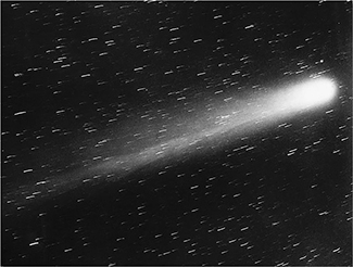
During the early 1600s, Johannes Kepler was able to use the amazingly accurate data from his mentor Tycho Brahe to formulate his three laws of planetary motion, now known as Kepler’s laws of planetary motion. These laws also apply to other objects in the solar system in orbit around the Sun, such as comets (e.g., Halley’s comet) and asteroids. Variations of these laws apply to satellites in orbit around Earth.
Theorem \PageIndex{3}: Kepler's Laws of Planetary Motion
- The path of any planet about the Sun is elliptical in shape, with the center of the Sun located at one focus of the ellipse (the law of ellipses).
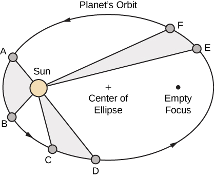
- A line drawn from the center of the Sun to the center of a planet sweeps out equal areas in equal time intervals (the law of equal areas) (Figure \PageIndex{4}).
- The ratio of the squares of the periods of any two planets is equal to the ratio of the cubes of the lengths of their semimajor orbital axes (the Law of Harmonies).
Kepler’s third law is especially useful when using appropriate units. In particular, 1 astronomical unit is defined to be the average distance from Earth to the Sun, and is now recognized to be 149,597,870,700 m or, approximately 93,000,000 mi. We therefore write 1 A.U. = 93,000,000 mi. Since the time it takes for Earth to orbit the Sun is 1 year, we use Earth years for units of time. Then, substituting 1 year for the period of Earth and 1 A.U. for the average distance to the Sun, Kepler’s third law can be written as
T_p^2=D_p^3
for any planet in the solar system, where T_P is the period of that planet measured in Earth years and D_P is the average distance from that planet to the Sun measured in astronomical units. Therefore, if we know the average distance from a planet to the Sun (in astronomical units), we can then calculate the length of its year (in Earth years), and vice versa.
Kepler’s laws were formulated based on observations from Brahe; however, they were not proved formally until Sir Isaac Newton was able to apply calculus. Furthermore, Newton was able to generalize Kepler’s third law to other orbital systems, such as a moon orbiting around a planet. Kepler’s original third law only applies to objects orbiting the Sun.
Proof
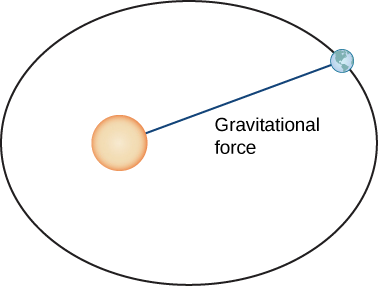
Let’s now prove Kepler’s first law using the calculus of vector-valued functions. First we need a coordinate system. Let’s place the Sun at the origin of the coordinate system and let the vector-valued function \vecs{r}(t) represent the location of a planet as a function of time. Newton proved Kepler’s law using his second law of motion and his law of universal gravitation. Newton’s second law of motion can be written as \vecs{F}=m\vecs{a}, where \vecs{F} represents the net force acting on the planet. His law of universal gravitation can be written in the form \vecs{F}=−\dfrac{GmM}{||\vecs{r}||^2}\cdot \dfrac{\vecs{r}}{||\vecs{r} ||}, which indicates that the force resulting from the gravitational attraction of the Sun points back toward the Sun, and has magnitude \dfrac{GmM}{||\vecs{r}||^2} (Figure \PageIndex{5}).
Setting these two forces equal to each other, and using the fact that \vecs a(t)=\vecs v′(t), we obtain
m\vecs v′(t)=−\frac{GmM}{‖\vecs r‖^2}⋅\frac{\vecs r}{‖\vecs r‖},
which can be rewritten as
\dfrac{d\vecs v}{dt}=−\dfrac{GM}{||\vecs r||^3}\vecs{r}.
This equation shows that the vectors d\vecs{v}/dt and \vecs r are parallel to each other, so d\vecs {v}/dt \times \vecs {r}=\vecs 0. Next, let’s differentiate \vecs{r} \times \vecs{v} with respect to time:
\dfrac{d}{dt}(\vecs{r}\times \vecs{v})=\dfrac{d\vecs{r}}{dt}\times \vecs v+\vecs{r} \times \dfrac{d\vecs{v}}{dt}=\vecs{v}\times \vecs{v}+\vecs{0}=\vecs{0}. \label{Eq10}
This proves that \vecs{r}\times\vecs{v} is a constant vector, which we call \vecs C. Since \vecs r and \vecs v are both perpendicular to \vecs C for all values of t, they must lie in a plane perpendicular to \vecs C. Therefore, the motion of the planet lies in a plane.
Next we calculate the expression d\vecs{v}/dt\times \vecs C:
\dfrac{d\vecs{v}}{dt} \times \vecs{C}=−\dfrac{GM}{||\vecs{r}||^3}\vecs{r}\times (\vecs{r}\times\vecs{v})=−\dfrac{GM}{||\vecs r||^3}[(\vecs{r} \cdot \vecs{v})\vecs{r} - (\vecs{r} \cdot \vecs{r})\vecs{v}]. \label{Eq11}
The last equality in Equation \ref{Eq11} is from the triple cross product formula (The Cross Product). We need an expression for \vecs{r}\cdot \vecs{v}. To calculate this, we differentiate \vecs{r}\cdot \vecs{r} with respect to time:
\dfrac{d}{dt}(\vecs{r}\cdot \vecs{r})=\dfrac{d\vecs{r}}{dt}\cdot \vecs{r}+\vecs{r}\cdot \dfrac{d\vecs{r}}{dt}=2\vecs{r}\cdot \dfrac{d\vecs{r}}{dt}=2\vecs{r}\cdot \vecs{v}. \label{Eq12}
Since \vecs{r}\cdot\vecs{r}=||\vecs r||^2, we also have
\dfrac{d}{dt}(\vecs{r}\cdot \vecs{r})=\dfrac{d}{dt}||\vecs{r}||^2=2||\vecs{r}|| \dfrac{d}{dt}||\vecs{r}||. \label{Eq13}
Combining Equation \ref{Eq12} and Equation \ref{Eq13}, we get
\begin{align*} 2\vecs{r}\cdot \vecs{v}&=2||\vecs{r}||\dfrac{d}{dt}||\vecs{r}|| \\[5pt] \vecs{r} \cdot \vecs{v} &=||\vecs{r}‖\dfrac{d}{dt}||\vecs{r}||. \end{align*} \label{Eq14}
Substituting this into Equation \ref{Eq11} gives us
\begin{align} \dfrac{d\vecs{v}}{dt} \times \vecs{C}&= - \dfrac{GM}{||\vecs{r}||^3} [(\vecs{r}\cdot \vecs{v})\vecs{r} - (\vecs{r}\cdot \vecs{r})\vecs{v}] \nonumber \\[5pt] &= -\dfrac{GM}{||\vecs{r}||^3}\left[ ||\vecs{r}|| \left(\dfrac{d}{dt} ||\vecs{r}||\right)\vecs{r} - ||\vecs{r}||^2\vecs{v} \right] \nonumber \\[5pt] &= -GM\left[ \dfrac{1}{||\vecs{r}||^2}\left( \dfrac{d}{dt} ||\vecs{r}|| \right)\vecs{r} - \dfrac{1}{||\vecs{r}||}\vecs{v} \right] \nonumber \\[5pt] &= GM\left[ \dfrac{\vecs{v}}{||\vecs{r}||} -\dfrac{\vecs{r}}{||\vecs{r}||^2}\left( \dfrac{d}{dt} ||\vecs{r}|| \right) \right]. \label{Eq15} \end{align}
However,
\begin{align*} \dfrac{d}{dt} \dfrac{\vecs{r}}{||\vecs{r}||} &= \dfrac{ \frac{d}{dt}(\vecs{r})||\vecs{r}||- \vecs{r}\frac{d}{dt}||\vecs{r}|| }{||\vecs{r}||^2} \\[5pt] &= \dfrac{ \frac{d\vecs{r}}{dt} }{||\vecs{r}||} - \dfrac{\vecs{r}}{||\vecs{r}||^2}\dfrac{d}{dt}||\vecs{r} || \\[5pt] &= \dfrac{\vecs{v}}{||\vecs{r}||} - \dfrac{\vecs{r}}{||\vecs{r}||^2} \dfrac{d}{dt}||\vecs{r}||. \end{align*}
Therefore, Equation \ref{Eq15} becomes
\dfrac{d \vecs{v}}{dt}\times \vecs{C}=GM\left( \dfrac{d}{dt}\dfrac{ \vecs{r}}{ || \vecs{r} ||} \right).
Since \vecs{C} is a constant vector, we can integrate both sides and obtain
\vecs{v}\times\vecs{C} = GM \dfrac{ \vecs{r} }{|| \vecs{r} ||} + \vecs{D},
where \vecs D is a constant vector. Our goal is to solve for || \vecs{r} ||. Let’s start by calculating \vecs{r} \cdot \left( \vecs{v}\times \vecs{C} \right):
\vecs{r} \cdot \left( \vecs{v}\times \vecs{C} \right) =GM\dfrac{||\vecs{r}||^2}{||\vecs{r}||}+ \vecs{r}\cdot\vecs{D} =GM||\vecs{r}||+\vecs{r}\cdot \vecs{D}.
However, \vecs{r} \cdot ( \vecs{v}\times \vecs{C})= ( \vecs{r} \times \vecs{v})\cdot \vecs{C} , so
( \vecs{r} \times \vecs{v})\cdot \vecs{C} =GM||\vecs{r}|| + \vecs{r}\cdot \vecs{D}.
Since \vecs{r}\times \vecs{v}=\vecs{C}, we have
||\vecs{C}||^2 =GM||\vecs{r}|| +\vecs{r}\cdot \vecs{D}.
Note that \vecs{r} \cdot \vecs{D}=||\vecs{r}|| ||\vecs{D}||\cos \theta , where \theta is the angle between \vecs{r} and \vecs{D}. Therefore,
||\vecs{C}||^2=GM||\vecs{r}||+||\vecs{r}|| ||\vecs{D}|| \cos\theta
Solving for ||\vecs{r}||,
||\vecs{r}|| = \dfrac{||\vecs{C}||^2 }{GM+||\vecs{D}||\cos\theta} = \dfrac{||\vecs{C}||^2}{GM}\left( \dfrac{1}{1+e\cos\theta} \right).
where e=||\vecs{D}||/GM. This is the polar equation of a conic with a focus at the origin, which we set up to be the Sun. It is a hyperbola if e>1, a parabola if e=1, or an ellipse if e<1. Since planets have closed orbits, the only possibility is an ellipse. However, at this point it should be mentioned that hyperbolic comets do exist. These are objects that are merely passing through the solar system at speeds too great to be trapped into orbit around the Sun. As they pass close enough to the Sun, the gravitational field of the Sun deflects the trajectory enough so the path becomes hyperbolic.
\square
Kepler’s third law of planetary motion can be modified to the case of one object in orbit around an object other than the Sun, such as the Moon around the Earth. In this case, Kepler’s third law becomes
P^2 = \dfrac{4\pi^2 a^3}{G(m+M)}, \label{Eq30}
where m is the mass of the Moon and M is the mass of Earth, a represents the length of the major axis of the elliptical orbit, and P represents the period.
Example \PageIndex{3}: Using Kepler’s Third Law for Nonheliocentric Orbits
Given that the mass of the Moon is 7.35\times 10^{22} kg, the mass of Earth is 5.97\times 10^{24} kg, G=6.67\times 10^{−11} \text{m} / \text{kg} \cdot \text{sec}^2, and the period of the moon is 27.3 days, let’s find the length of the major axis of the orbit of the Moon around Earth.
Solution
It is important to be consistent with units. Since the universal gravitational constant contains seconds in the units, we need to use seconds for the period of the Moon as well:
27.3 \; \text{days} \times \dfrac{24 \; \text{hr}}{1 \; \text{day}} \times \dfrac{3600 \; \text{sec}}{1 \; \text{hour}} =2,358,720\; \text{sec}
Substitute all the data into Equation \ref{Eq30} and solve for a:
\begin{align*} (2,358,720 \; \text{sec})^2 &= \dfrac{4\pi^2a^3}{\left( 6.67\times 10^{-11} \frac{m}{\text{kg}\times \text{sec}^2}\right) (7.35\times 10^{22}\text{kg} + 5.97 \times 10^{24}\text{kg})} \\[5pt] 5.563 \times 10^{12} &= \dfrac{ 4\pi^2a^3}{(6.67 \times 10^{-11}\text{m}^3)(6.04 \times 10^{24})} \\[5pt] (5.563 \times 10^{12})(6.67 \times 10^{-11} \text{m}^3)(6.04 \times 10^{24}) &= 4\pi^2 a^3 \\[5pt] a^3 &= \dfrac{2.241 \times 10^{27}}{4\pi^2}\text{m}^3 \\[5pt] a&= 3.84 \times 10^8 \text{m} \\[5pt] &\approx 384,000 \,\text{km}. \end{align*}
Analysis
According to solarsystem.nasa.gov, the actual average distance from the Moon to Earth is 384,400 km. This is calculated using reflectors left on the Moon by Apollo astronauts back in the 1960s.
Exercise \PageIndex{3}
Titan is the largest moon of Saturn. The mass of Titan is approximately 1.35 \times 10^{23} kg. The mass of Saturn is approximately 5.68 \times 10^{26} kg. Titan takes approximately 16 days to orbit Saturn. Use this information, along with the universal gravitation constant G=6.67×10^{−11} \text{m}/\text{kg} \cdot \text{sec}^2 to estimate the distance from Titan to Saturn.
- Hint
-
Make sure your units agree, then use Equation \ref{Eq30}.
- Answer
-
a\approx 1.224 \times 10^9 \text{m}= 1,224,000 \text{km}
Example \PageIndex{4}: Halley’s Comet
We now return to the chapter opener, which discusses the motion of Halley’s comet around the Sun. Kepler’s first law states that Halley’s comet follows an elliptical path around the Sun, with the Sun as one focus of the ellipse. The period of Halley’s comet is approximately 76.1 years, depending on how closely it passes by Jupiter and Saturn as it passes through the outer solar system. Let’s use T=76.1 years. What is the average distance of Halley’s comet from the Sun?
Solution
Using the equation T^2=D^3 with T=76.1, we obtain D^3=5791.21, so D\approx 17.96 A.U. This comes out to approximately 1.67\times 10^9 mi.
A natural question to ask is: What are the maximum (aphelion) and minimum (perihelion) distances from Halley’s Comet to the Sun? The eccentricity of the orbit of Halley’s Comet is 0.967 (Source: http://nssdc.gsfc.nasa.gov/planetary...cometfact.html). Recall that the formula for the eccentricity of an ellipse is e=c/a, where a is the length of the semimajor axis and c is the distance from the center to either focus. Therefore, 0.967=c/17.96 and c\approx 17.37 A.U. Subtracting this from a gives the perihelion distance p=a−c=17.96−17.37=0.59 A.U. According to the National Space Science Data Center (Source: http://nssdc.gsfc.nasa.gov/planetary...cometfact.html), the perihelion distance for Halley’s comet is 0.587 A.U. To calculate the aphelion distance, we add
P=a+c=17.96+17.37=35.33 \; \text{A.U.}
This is approximately 3.3\times 10^9 mi. The average distance from Pluto to the Sun is 39.5 A.U. (Source: http://www.oarval.org/furthest.htm), so it would appear that Halley’s Comet stays just within the orbit of Pluto.
NAVIGATING A BANKED TURN
How fast can a racecar travel through a circular turn without skidding and hitting the wall? The answer could depend on several factors:
- The weight of the car;
- The friction between the tires and the road;
- The radius of the circle;
- The “steepness” of the turn.
In this project we investigate this question for NASCAR racecars at the Bristol Motor Speedway in Tennessee. Before considering this track in particular, we use vector functions to develop the mathematics and physics necessary for answering questions such as this.
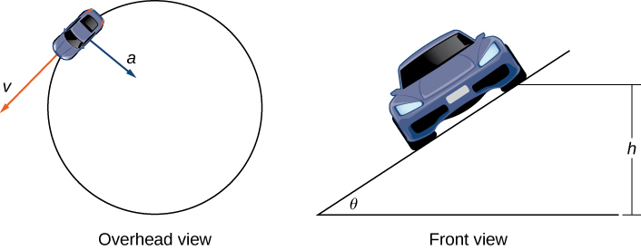
A car of mass m moves with constant angular speed \omega around a circular curve of radius R (Figure \PageIndex{7}). The curve is banked at an angle \theta. If the height of the car off the ground is h, then the position of the car at time t is given by the function \vecs r(t)=< R\cos(\omega t),R\sin(\omega t),h>.
- Find the velocity function \vecs{v}(t) of the car. Show that \vecs{v} is tangent to the circular curve. This means that, without a force to keep the car on the curve, the car will shoot off of it.
- Show that the speed of the car is \omega R. Use this to show that (2\pi 4)/\|\vecs{v}\|=(2\pi)/\omega .
- Find the acceleration \vecs{a}. Show that this vector points toward the center of the circle and that \|\vecs{a}\|=R\omega ^2.
- The force required to produce this circular motion is called the centripetal force, and it is denoted \vecs{F}_{cent} . This force points toward the center of the circle (not toward the ground). Show that \|\vecs{F}_{cent}\|=\left(m|\vecs{v}|^2 \right)/R.
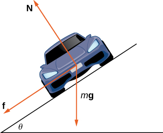
As the car moves around the curve, three forces act on it: gravity, the force exerted by the road (this force is perpendicular to the ground), and the friction force (Figure \PageIndex{8}). Because describing the frictional force generated by the tires and the road is complex, we use a standard approximation for the frictional force. Assume that \vecs{f}=\mu \vecs{N} for some positive constant \mu . The constant \mu is called the coefficient of friction.
Let v_{max} denote the maximum speed the car can attain through the curve without skidding. In other words, v_{max} is the fastest speed at which the car can navigate the turn. When the car is traveling at this speed, the magnitude of the centripetal force is
\| \vecs{F}_{cent} \| = \dfrac{m(v_{max})^2}{R}.
The next three questions deal with developing a formula that relates the speed v_{max} to the banking angle \theta.
- Show that \vecs{N} \cos\theta=m\vecs g+\vecs{f} \sin\theta. Conclude that \vecs{N}=(m\vecs g)/(\cos\theta−\mu \sin\theta).
- The centripetal force is the sum of the forces in the horizontal direction, since the centripetal force points toward the center of the circular curve. Show that
\vecs{F}_{cent}=\vecs{N} \sin\theta+\vecs{f}\cos\theta.
Conclude that\vecs{F}_{cent}=\dfrac{\sin\theta+\mu \cos\theta}{cos\theta−\mu \sin\theta} m\vecs g.
- Show that (v_{\text{max}})^2=((\sin\theta+\mu\ cos\theta)/(\cos\theta−\mu \sin\theta))gR. Conclude that the maximum speed does not actually depend on the mass of the car.
Now that we have a formula relating the maximum speed of the car and the banking angle, we are in a position to answer the questions like the one posed at the beginning of the project.
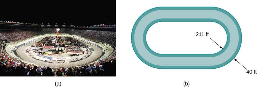
The Bristol Motor Speedway is a NASCAR short track in Bristol, Tennessee. The track has the approximate shape shown in Figure \PageIndex{9}. Each end of the track is approximately semicircular, so when cars make turns they are traveling along an approximately circular curve. If a car takes the inside track and speeds along the bottom of turn 1, the car travels along a semicircle of radius approximately 211 ft with a banking angle of 24°. If the car decides to take the outside track and speeds along the top of turn 1, then the car travels along a semicircle with a banking angle of 28°. (The track has variable angle banking.)
The coefficient of friction for a normal tire in dry conditions is approximately 0.7. Therefore, we assume the coefficient for a NASCAR tire in dry conditions is approximately 0.98.
Before answering the following questions, note that it is easier to do computations in terms of feet and seconds, and then convert the answers to miles per hour as a final step.
- In dry conditions, how fast can the car travel through the bottom of the turn without skidding?
- In dry conditions, how fast can the car travel through the top of the turn without skidding?
- In wet conditions, the coefficient of friction can become as low as 0.1. If this is the case, how fast can the car travel through the bottom of the turn without skidding?
- Suppose the measured speed of a car going along the outside edge of the turn is 105 mph. Estimate the coefficient of friction for the car’s tires.
Key Concepts
- The acceleration vector always points toward the concave side of the curve defined by \vecs{r}(t). The tangential and normal components of acceleration a_\vecs{T} and a_\vecs{N} are the projections of the acceleration vector onto the unit tangent and unit normal vectors to the curve.
- Kepler’s three laws of planetary motion describe the motion of objects in orbit around the Sun. His third law can be modified to describe motion of objects in orbit around other celestial objects as well.
- Newton was able to use his law of universal gravitation in conjunction with his second law of motion and calculus to prove Kepler’s three laws.
Key Equations
- Tangential component of acceleration a_{\vecs{T}} =\vecs{a}\cdot \vecs{T}=\dfrac{\vecs{v}\cdot \vecs{a}}{||\vecs v||} \nonumber
- Normal component of acceleration a_{\vecs{N}}=\vecs{a}\cdot \vecs{N} = \dfrac{|| \vecs{v} \times \vecs{a} ||}{||\vecs{v}||} = \sqrt{||\vecs{a}||^2 - \left(a_{\vecs{T}}\right)^2} \nonumber
Glossary
- acceleration vector
- the second derivative of the position vector
- Kepler’s laws of planetary motion
- three laws governing the motion of planets, asteroids, and comets in orbit around the Sun
- normal component of acceleration
- the coefficient of the unit normal vector \vecs N when the acceleration vector is written as a linear combination of \vecs T and \vecs N
- tangential component of acceleration
- the coefficient of the unit tangent vector \vecs T when the acceleration vector is written as a linear combination of \vecs T and \vecs N
Contributors
Gilbert Strang (MIT) and Edwin “Jed” Herman (Harvey Mudd) with many contributing authors. This content by OpenStax is licensed with a CC-BY-SA-NC 4.0 license. Download for free at http://cnx.org.
- Paul Seeburger added Figure \PageIndex{1}, Exercise \PageIndex{1}, the exposition below Figure \PageIndex{1} through Theorem \PageIndex{3}, and from Example \PageIndex{2} until just before Kepler's Laws.