4.1: Parametric Equations

Learning Objectives

• Plot a curve described by parametric equations.
• Convert the parametric equations of a curve into the form $y=f(x)$.
• Recognize the parametric equations of basic curves, such as a line and a circle.
• Recognize the parametric equations of a cycloid.

Parametric Equations and Their Graphs

Consider the orbit of Earth around the Sun. Our year lasts approximately 365.25 days, but for this discussion, we will use 365 days. On January 1 of each year, the physical location of Earth with respect to the Sun is nearly the same, except for leap years, when the lag introduced by the extra $\frac{1}{4}$ day of orbiting time is built into the calendar. We call January 1 “day 1” of the year. Then, for example, day 31 is January 31, day 59 is February 28, and so on.

The number of the day in a year can be considered a variable that determines Earth’s position in its orbit. As Earth revolves around the Sun, its physical location changes relative to the Sun. After one full year, we are back where we started, and a new year begins. According to Kepler’s laws of planetary motion, the shape of the orbit is elliptical, with the Sun at one focus of the ellipse. We study this idea in more detail in Conic Sections.

Figure $\PageIndex{1}$: Earth’s orbit around the Sun during one year. The point labeled $F_2$ is one of the foci of the ellipse; the other focus is occupied by the Sun. In the figure, an ellipse with January 1 ( $t = 1$) at the top, April 2 ( $t = 92$) on the left, July 1 ( $t = 182$) on the bottom, and October 1 ( $t = 274$) on the right. The focal points of the ellipse have F2 on the left and the Sun on the right.

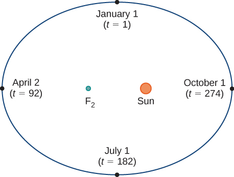
If we superimpose coordinate axes over this graph, then we can assign ordered pairs to each point on the ellipse Figure $\PageIndex{2}$. Then each $x$ value on the graph is a value of position as a function of time, and each $y$ value is also a value of position as a function of time. Therefore, each point on the graph corresponds to a value of Earth’s position as a function of time.

Figure $\PageIndex{2}$: Coordinate axes superimposed on the orbit of Earth from Figure $\PageIndex{1}$ with the origin at the center of the ellipse.

We can determine the functions for $x(t)$ and $y(t)$, thereby parameterizing the orbit of Earth around the Sun. The variable $t$ is called an independent parameter and, in this context, represents time relative to the beginning of each year.

A curve in the $(x,y)$ plane can be represented parametrically. The equations that are used to define the curve are called parametric equations.

Definition: Parametric Equations

If $x$ and $y$ are continuous functions of $t$ on an interval $I$, then the equations

$$x=x(t)$$

and

$$y=y(t)$$

are called parametric equations and $t$ is called the parameter. The set of points $(x,y)$ obtained as $t$ varies over the interval $I$ is called the graph of the parametric equations. The graph of parametric equations is called a parametric curve or plane curve, and is denoted by $C$.

Notice in this definition that $x$ and $y$ are used in two ways. The first is as functions of the independent variable $t$. As $t$ varies over the interval $I$, the functions $x(t)$ and $y(t)$ generate a set of ordered pairs $(x,y)$. This set of ordered pairs generates the graph of the parametric equations. In this second usage, to designate the ordered pairs, $x$ and $y$ are variables. It is important to distinguish the variables $x$ and $y$ from the functions $x(t)$ and $y(t)$.

Example $\PageIndex{1}$: Graphing a Parametrically Defined Curve

Sketch the curves described by the following parametric equations:

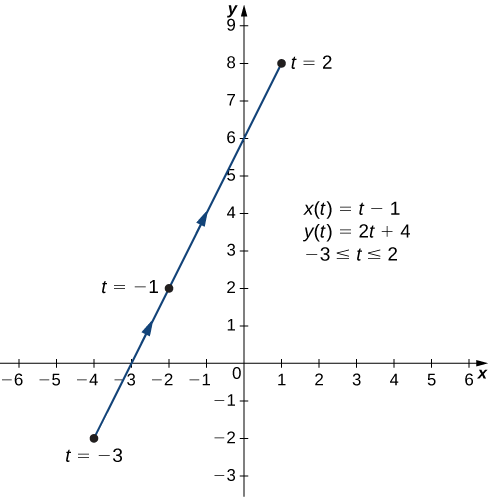
1. $x(t)=t−1, \quad y(t)=2t+4,\quad \text{for }−3≤t≤2$
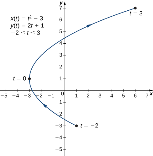
2. $x(t)=t^2−3, \quad y(t)=2t+1,\quad \text{for }−2≤t≤3$
3. $x(t)=4 \cos t, \quad y(t)=4 \sin t,\quad \text{for }0≤t≤2π$

Solution

1. First, set up a table (Table $\PageIndex{1}$) of values to create a graph of this curve. Since the independent variable in both $x(t)$ and $y(t)$ is $t$, let $t$ appear in the first column. Then $x(t)$ and $y(t)$ will appear in the second and third columns of the table.

Table $\PageIndex{1}$: Values of parametric equations $x(t)=t-1$ and $y(t)=2t+4$ over $-3 \le t \le 2$

$t$	$x(t)$	$y(t)$
−3	−4	−2
−2	−3	0
−1	−2	2
0	−1	4
1	0	6
2	1	8

The second and third columns in this table provide a set of points to be plotted. The graph of these points appears in Figure $\PageIndex{3}$. The arrows on the graph indicate the orientation of the graph, that is, the direction that a point moves on the graph as $t$ varies from $−3$ to $2$.

Figure $\PageIndex{3}$: Graph of the plane curve described by the parametric equations in Example $\PageIndex{1}$, part a. A straight line going from (−4, −2) through (−3, 0), (−2, 2), and (0, 6) to (1, 8) with an arrow pointed up and to the right. The point (−4, −2) is marked $t = −3$, the point (−2, 2) is marked $t = −1$, and the point (1, 8) is marked $t = 2$.

b. To create a graph of this curve, again set up a table of values.

Table $\PageIndex{2}$: Values of parametric equations $x(t)=t^2-3$ and $y(t)=2t+1$ over $-2 \le t \le 3$

$t$	$x(t)$	$y(t)$
−2	1	−3
−1	−2	−1
0	−3	1
1	−2	3
2	1	5
3	6	7

The second and third columns in this table give a set of points to be plotted (Figure $\PageIndex{4}$). The first point on the graph (corresponding to $t=−2$) has coordinates $(1,−3)$, and the last point (corresponding to $t=3$) has coordinates $(6,7)$. As $t$ progresses from $−2$ to $3$, the point on the curve travels along a parabola. The direction the point moves is again called the orientation and is indicated on the graph.

Figure $\PageIndex{4}$: Graph of the plane curve described by the parametric equations Example $\PageIndex{1}$, part b. A curved line going from (1, −3) through (−3, 1) to (6, 7) with arrow pointing in that order. The point (1, −3) is marked $t = −2$, the point (−3, 1) is marked $t = 0$, and the point (6, 7) is marked $t = 3$.

c. In this case, use multiples of $π/6$ for $t$ and create another table of values:

Table $\PageIndex{3}$: Values of parametric equations $x(t) = 4 \cos t , y(t) = 4 \sin t$ over $0 \le t \le 2\pi$

$t$	$x(t)$	$y(t)$	$t$	$x(t)$	$y(t)$
0	4	0	$\frac{7π}{6}$	$-2\sqrt{3}≈−3.5$	-2
$\frac{π}{6}$	$2\sqrt{3}≈3.5$	2	$\frac{4π}{3}$	−2	$−2\sqrt{3}≈−3.5$
$\frac{π}{3}$	2	$2\sqrt{3}≈3.5$	$\frac{3π}{2}$	0	−4
$\frac{π}{2}$	0	4	$\frac{5π}{3}$	2	$−2\sqrt{3}≈−3.5$
$\frac{2π}{3}$	−2	$2\sqrt{3}≈3.5$	$\frac{11π}{6}$	$2\sqrt{3}≈3.5$	-2
$\frac{5π}{6}$	$−2\sqrt{3}≈−3.5$	2	$2π$	4	0
$π$	−4	0

The graph of this plane curve appears in the following graph, Figure $\PageIndex{5}$.

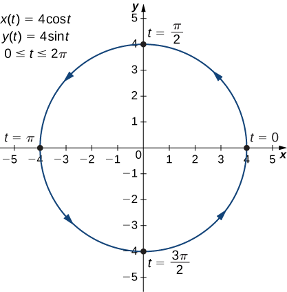
Figure $\PageIndex{5}$: Graph of the plane curve described by the parametric equations in Example $\PageIndex{1}$, part c. This is the graph of a circle with radius $4$ centered at the origin, with a counterclockwise orientation. The point (4, 0) is marked $t = 0$, the point (0, 4) is marked $t = \pi/2$, the point (−4, 0) is marked $t = \pi$, and the point (0, −4) is marked $t = 3\pi/2$. The starting point and ending points of the curve both have coordinates $(4,0)$.

Exercise $\PageIndex{1}$

Sketch the curve described by the parametric equations

$$x(t)=3t+2,\quad y(t)=t^2−1,\quad \text{for }−3≤t≤2. \nonumber$$

Hint

Make a table of values for $x(t)$ and $y(t)$ using $t$ values from $−3$ to $2$.

Answer

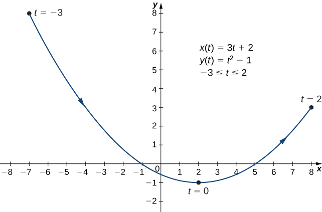
Figure $\PageIndex{6}$: On the graph there are also written three equations: $x(t) = 3t + 2, y(t) = t^2 − 1$, and $−3 ≤ t ≤ 2$. A curved line going from (−7, 8) through (−1, 0) and (2, −1) to (8, 3) with an arrow going in that order. The point (−7, 8) is marked $t = −3$, the point (2, −1) is marked $t = 0$, and the point (8, 3) is marked $t = 2$.

Interactive Element

Visualizing a Parametric Curves As Time Elapses

Unlike curves that are described in the form $y=f(x)$ that just give the static path of an object, parametrically described curves, $x=x(t), y = y(t)$, give the dynamic motion of an object. The visualization below shows the graph of the static curve defined parametrically, but if you click on the "Move" button, you can observe its dynamic motion by observing the dynamic motion of an ant as it travels according to the motion described by the parametrically defined path.  If you click on the Next button, it will take you to a different parametrically defined curve.

$x(t)=\sin(t), y(t)=2\sin(t), 0<t<20$

$x(t)=t^2, y(t)=t^3, -2<t<2$

$x(t)=\cos(-t), y(t)=\sin(-t), 0<t<20$

$x(t)=e^t, y(t)=e^{2t}, -2<t<1$

$x(t)=t^3-6t, y(t)=t^2-5, 0<t<3$

$x(t)=t-\sin(t), y(t)=1-\cos(t), 0<t<10$

$x(t)=2\cos(t^2), y(t)=2\sin(t^2), 0<t<8$

$x(t)=e^t\cos(8t), y(t)=e^t\sin(8t), -2<t<2$

$x(t)=\frac{1}{t}, y(t)=\frac{1}{t^2}, -4<t<4$

$x(t)=t+t^2, y(t)=t-t^2, -3<t<3$

Move  Next

 

Eliminating the Parameter

To better understand the graph of a curve represented parametrically, it is useful to rewrite the two equations as a single equation relating the variables $x$ and $y$. Then we can apply any previous knowledge of equations of curves in the plane to identify the curve. For example, the equations describing the plane curve in Example $\PageIndex{1b}$ are

$$\begin{align} x(t) &=t^2−3 \label{x1} \\[4pt] y(t) &=2t+1 \label{y1} \end{align}$$

over the region $-2 \le t \le 3.$

Solving (Equation 4.1.4) for $t$ gives

$$t=\dfrac{y−1}{2}. \nonumber$$

This can be substituted into (Equation 4.1.3):

$$\begin{align} x &=\left(\dfrac{y−1}{2}\right)^2−3 \\[4pt] &=\dfrac{y^2−2y+1}{4}−3 \\[4pt] &=\dfrac{y^2−2y−11}{4}. \label{y2}\end{align}$$

(Equation 4.1.7) describes $x$ as a function of $y$. These steps give an example of eliminating the parameter. The graph of this function is a parabola opening to the right Figure $\PageIndex{4}$. Recall that the plane curve started at $(1,−3)$ and ended at $(6,7)$. These terminations were due to the restriction on the parameter $t$.

Example $\PageIndex{2}$: Eliminating the Parameter

Eliminate the parameter for each of the plane curves described by the following parametric equations and describe the resulting graph.

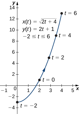
1. $x(t)=\sqrt{2t+4}, \quad y(t)=2t+1,\quad \text{for }−2≤t≤6$
2. $x(t)=4\cos t, \quad y(t)=3\sin t,\quad \text{for }0≤t≤2π$

Solution

1. To eliminate the parameter, we can solve either of the equations for $t$. For example, solving the first equation for $t$ gives

$$\begin{align*} x &=\sqrt{2t+4} \\[4pt] x^2 &=2t+4 \\[4pt] x^2−4 &=2t \\[4pt] t &=\dfrac{x^2−4}{2}. \end{align*}$$

Note that when we square both sides it is important to observe that $x≥0$. Substituting $t=\dfrac{x^2−4}{2}$ into $y(t)$ yields

$$y(t)=2t+1$$

$$y=2\left(\dfrac{x^2−4}{2}\right)+1$$

$$y=x^2−4+1$$

$$y=x^2−3.$$

This is the equation of a parabola opening upward. There is, however, a domain restriction because of the limits on the parameter $t$. When $t=−2$, $x=\sqrt{2(−2)+4}=0$, and when $t=6$, $x=\sqrt{2(6)+4}=4$. The graph of this plane curve follows.

Figure $\PageIndex{7}$: Graph of the plane curve described by the parametric equations. A curved line is going from (−3, 0) through (2, 1) to (4, 13) with an arrow going in that order. The point (−3, 0) is marked $t = −2$, the point (2, 1) is marked $t = 0$, the point (2 times the square root of 2, 5) is marked $t = 2$, the point (3 times the square root of 2, 9) is marked $t = 4$, and the point (4, 13) is marked $t = 6$.

Watch the accompanying video for a visual demonstration of this concept.

• Video Length: 1 minute 45 seconds
• Context: This video demonstrates how to graph a parametric curve after eliminating the parameter from the equations $x(t)=e^t, y(t)=(e^t)^2$, showcasing techniques for handling exponential functions in calculus.

2. Sometimes it is necessary to be a bit creative in eliminating the parameter. The parametric equations for this example are

$$x(t)=4 \cos t\nonumber$$

and

$$y(t)=3 \sin t\nonumber$$

Solving either equation for $t$ directly is not advisable because sine and cosine are not one-to-one functions. However, dividing the first equation by $4$ and the second equation by $3$ (and suppressing the $t$) gives us

$$\cos t=\dfrac{x}{4}\nonumber$$

and

$$\sin t=\dfrac{y}{3}.\nonumber$$

Now use the Pythagorean identity $\cos^2t+\sin^2t=1$ and replace the expressions for $\sin t$ and $\cos t$ with the equivalent expressions in terms of $x$ and $y$. This gives

$$\left(\dfrac{x}{4}\right)^2+\left(\dfrac{y}{3}\right)^2=1 \nonumber$$

$$\dfrac{x^2}{16}+\dfrac{y^2}{9}=1. \nonumber$$

This is the equation of a horizontal ellipse centered at the origin, with semi-major axis $4$ and semi-minor axis $3$ as shown in the following graph.

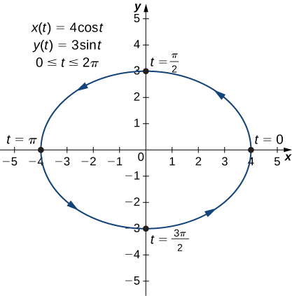
Figure $\PageIndex{8}$: Graph of the plane curve described by the parametric equations: $x(t) = 4 \cos(t)$, $y(t) = \sin(t)$, and $0 \le t \le 2\pi$. An ellipse with horizontal major axis of length 8 and with vertical minor radius length 6 that is centered at the origin with an arrow going counterclockwise. The point $(4, 0)$ is marked $t = 0$, the point $(0, 3)$ is marked $t = \pi/2$, the point $(−4, 0)$ is marked $t = \pi$, and the point $(0, −3)$ is marked $t = 3\pi/2$.

As t progresses from $0$ to $2π$, a point on the curve traverses the ellipse once, in a counterclockwise direction. Recall from the section opener that the orbit of Earth around the Sun is also elliptical. This is a perfect example of using parameterized curves to model a real-world phenomenon.

Watch the accompanying video for a visual demonstration of this concept.

• Video Length: 2 minutes 24 seconds.
• Context: This video demonstrates how to graph a parametric curve after eliminating the parameter of the equations $x=2\sin\theta$, $y=2\cos\theta$, showcasing techniques for handling trigonometric functions in calculus.

Exercise $\PageIndex{2}$

Eliminate the parameter for the plane curve defined by the following parametric equations and describe the resulting graph.

$$x(t)=2+\dfrac{3}{t}, \quad y(t)=t−1, \quad\text{for }2≤t≤6 \nonumber$$

Hint

Solve one of the equations for $t$ and substitute into the other equation.

Answer

$x=2+\frac{3}{y+1},$ or $y=−1+\frac{3}{x−2}$. This equation describes a portion of a rectangular hyperbola centered at $(2,−1)$.The point (3.5, 1) is marked $t = 2$ and the point (2.5, 5) is marked $t = 6$.

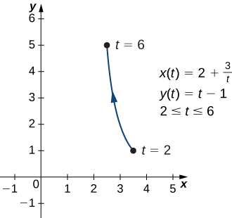
Figure $\PageIndex{9}$: Equations: $x(t) = 2 + 3/t, y(t) = t − 1$, and $2 \le t \le 6$. A curved line going from $(3.5, 1)$ to $(2.5, 5)$ with an arrow going in that order.

So far we have seen the method of eliminating the parameter, assuming we know a set of parametric equations that describe a plane curve. What if we would like to start with the equation of a curve and determine a pair of parametric equations for that curve? This is certainly possible, and in fact, it is possible to do so in many different ways for a given curve. The process is known as the parameterization of a curve.

Example $\PageIndex{3}$

Find two different pairs of parametric equations to represent the graph of $y=2x^2−3$.

Solution

First, it is always possible to parameterize a curve by defining $x(t)=t$, then replacing $x$ with $t$ in the equation for $y(t)$. This gives the parameterization

$$x(t)=t, \quad y(t)=2t^2−3. \nonumber$$

Since there is no restriction on the domain in the original graph, there is no restriction on the values of $t$.

We have complete freedom in the choice for the second parameterization. For example, we can choose $x(t)=3t−2$. The only thing we need to check is that there are no restrictions imposed on $x$; that is, the range of $x(t)$ is all real numbers. This is the case for $x(t)=3t−2$. Now since $y=2x^2−3$, we can substitute $x(t)=3t−2$ for $x$. This gives

$$y(t)=2(3t−2)^2−2=2(9t^2−12t+4)−2=18t^2−24t+8−2=18t^2−24t+6. \nonumber$$

Therefore, a second parameterization of the curve can be written as

$x(t)=3t−2$ and $y(t)=18t^2−24t+6.$

Exercise $\PageIndex{3}$

Find two different sets of parametric equations to represent the graph of $y=x^2+2x$.

Hint

Follow the steps in Example $\PageIndex{3}$. Remember we have freedom in choosing the parameterization for $x(t)$.

Answer

One possibility is $x(t)=t, \quad y(t)=t^2+2t.$ Another possibility is $x(t)=2t−3, \quad y(t)=(2t−3)^2+2(2t−3)=4t^2−8t+3.$ There are, in fact, an infinite number of possibilities.

The video examples below start with the equation of a curve, and determine a pair of parametric equations for a line, a function, a circle, and the intersection of parametric curves.

Example $\PageIndex{4}$

Find parametric equations of the line that passes through the points $(3, 4)$ and $(1, 7)$.

Solution

• Video Length: 3 minutes 27 seconds
• Context: This video demonstrates how to find parametric equations of a line involves expressing the coordinates of points on the line as functions of a parameter, usually by defining the x, y, and z components (in 3D) or x and y components (in 2D) based on a point the line passes through and a direction vector.

Example $\PageIndex{5}$

Find parametric equations for the curve represented by $f(x)=e^x - \sin x$.

Solution

• Video Length: 50 seconds
• Context: This video demonstrates writing the parametric equation of a function $f(x)=e^x-\sin x$, showcasing techniques for handling exponential and trigonometric functions in calculus.

Example $\PageIndex{6}$

Find the parametric equations of a circle centered at $(2, -3)$ with radius 4.

Solution

• Video Length: 1 minute 35 seconds.
• Context: This video demonstrates writing parametric equations of a circle by writing the relation between the rectangular and polar coordinates. The process typically involves using trigonometric functions to describe the $x$ and $y$ coordinates of a point on the circle in terms of a parameter, usually denoted as $\theta$.

Example $\PageIndex{7}$

Finding the parametric equations to the line through the point $(2,-1,3)$ that is parallel to the line

$$x=2-t, y=1+2t, z=3+5t\nonumber$$

Solution

• Video Length: 2 minutes 22 seconds.
• Context: This video demonstrates writing the parametric equations of a line passing through a point and parallel to the given line. The parametric equations are derived by starting from the point P_0​ and adding a scaled version of the direction vector v, controlled by a parameter t.

Example $\PageIndex{8}$

Determining given lines intersect. If they do find the point of the intersection.

$$x=3-2t, y=4 +t, z=-2+5t\nonumber$$

$$x=-t, y=7-t, z=-1+9t\nonumber$$

Solution

• Video Length: 5 minutes 35 seconds.
• Context: This video demonstrates how to find the point of intersection of the parametric equations.

Cycloids and Other Parametric Curves

Imagine going on a bicycle ride through the country. The tires stay in contact with the road and rotate in a predictable pattern. Now suppose a very determined ant is tired after a long day and wants to get home. So he hangs onto the side of the tire and gets a free ride. The path that this ant travels down a straight road is called a cycloid Figure $\PageIndex{10}$. A cycloid generated by a circle (or bicycle wheel) of radius a is given by the parametric equations

$$x(t)=a(t−\sin t), \quad y(t)=a(1−\cos t).\nonumber$$

To see why this is true, consider the path that the center of the wheel takes. The center moves along the $x$-axis at a constant height equal to the radius of the wheel. If the radius is $a$, then the coordinates of the center can be given by the equations

$$x(t)=at,\quad y(t)=a\nonumber$$

for any value of $t$. Next, consider the ant, which rotates around the center along a circular path. If the bicycle is moving from left to right then the wheels are rotating in a clockwise direction. A possible parameterization of the circular motion of the ant (relative to the center of the wheel) is given by

$$\begin{align*} x(t) &=−a \sin t \\[4pt] y(t) &=−a\cos t.\end{align*}$$

(The negative sign is needed to reverse the orientation of the curve. If the negative sign were not there, we would have to imagine the wheel rotating counterclockwise.) Adding these equations together gives the equations for the cycloid.

$$\begin{align*} x(t) &=a(t−\sin t) \\[4pt] y(t) &=a(1−\cos t ) \end{align*}$$

Figure $\PageIndex{10}$ shows a series of circles with a center marked and a point on the circle drawing out a curve as if the circle was rolling along a plane. The shape made seems to be half an ellipse with the height the diameter of the original circle and with major axis the circumference of the circle.

Figure $\PageIndex{10}$: A wheel traveling along a road without slipping; the point on the edge of the wheel traces out a cycloid.

Now suppose that the bicycle wheel doesn’t travel along a straight road but instead moves along the inside of a larger wheel, as in (Figure $\PageIndex{11}$). Two circles are drawn both with center at the origin and with radii $3$ and $4$, respectively; the circle with radius $3$ has an arrow pointing in the counterclockwise direction. There is a third circle drawn with the center on the circle with radius $3$ and touching the circle with radius $4$ at one point. That is, this third circle has radius equal to $1$. A point is drawn on this third circle, and if it were to roll along the other two circles, it would draw out a four pointed star with points at $(4, 0)$, $(0, 4)$, $(−4, 0)$, and $(0, −4)$. In this graph, the green circle is traveling around the blue circle in a counterclockwise direction. A point on the edge of the green circle traces out the red graph, which is called a hypocycloid.

Figure $\PageIndex{11}$: Graph of the hypocycloid described by the parametric equations $x(t) = 3 cos(t) + cos(3t)$ and $y(t) = 3 sin(t) – sin(3t)$.

The general parametric equations for a hypocycloid are

$$x(t)=(a−b) \cos t+b \cos (\dfrac{a−b}{b})t \nonumber$$

$$y(t)=(a−b) \sin t−b \sin (\dfrac{a−b}{b})t. \nonumber$$

These equations are a bit more complicated, but the derivation is somewhat similar to the equations for the cycloid. In this case we assume the radius of the larger circle is $a$ and the radius of the smaller circle is $b$. Then the center of the wheel travels along a circle of radius $a−b.$ This fact explains the first term in each equation above. The period of the second trigonometric function in both $x(t)$ and $y(t)$ is equal to $\dfrac{2πb}{a−b}$.

The ratio $\dfrac{a}{b}$ is related to the number of cusps on the graph (cusps are the corners or pointed ends of the graph), as illustrated in Figure $\PageIndex{12}$. This ratio can lead to some very interesting graphs, depending on whether or not the ratio is rational. Figure $\PageIndex{11}$ corresponds to $a=4$ and $b=1$. The result is a hypocycloid with four cusps. Figure $\PageIndex{12}$ shows some other possibilities. The last two hypocycloids have irrational values for $\dfrac{a}{b}$. In these cases the hypocycloids have an infinite number of cusps, so they never return to their starting point. These are examples of what are known as space-filling curves.

Figure $\PageIndex{12}$: Graph of various hypocycloids corresponding to different values of $a/b$. A series of hypocycloids is given.

In the Figure $\PageIndex{12}$ first is a three pointed star marked $\frac{a}{b} = 3$. The second is a four pointed star marked $\frac{a}{b} = 4$. The third is a five pointed star marked $\frac{a}{b} = 5$. None of these first three figures has lines that cross each other. The fourth figure is a five pointed star but this one has lines which cross each other and looks like the star that children first learn to draw; it is marked $\frac{a}{b} = 5/3$. A similar sort of star with seven points is next and is marked $\frac{a}{b} = 7/3$. Then a similar star with eight points is next and is marked $\frac{a}{b} = 8/3$. The next figure is a complicated series of curves that ultimately creates a small rosette in the middle; this is marked $\frac{a}{b} = π$. Lastly, there is an even more complicated series of curves that creates a large rosette with sharper florets marked $\frac{a}{b} = \sqrt{2}$.

The Witch of Agnesi

Many plane curves in mathematics are named after the people who first investigated them, like the folium of Descartes or the spiral of Archimedes. However, perhaps the strangest name for a curve is the witch of Agnesi. Why a witch?

Maria Gaetana Agnesi (1718–1799) was one of the few recognized women mathematicians of eighteenth-century Italy. She wrote a popular book on analytic geometry, published in 1748, which included an interesting curve that had been studied by Fermat in 1630. The mathematician Guido Grandi showed in 1703 how to construct this curve, which he later called the “versoria,” a Latin term for a rope used in sailing. Agnesi used the Italian term for this rope, “versiera,” but in Latin, this same word means a “female goblin.” When Agnesi’s book was translated into English in 1801, the translator used the term “witch” for the curve, instead of rope. The name “witch of Agnesi” has stuck ever since.

The witch of Agnesi is a curve defined as follows: Start with a circle of radius a so that the points $(0,0)$ and $(0,2a)$ are points on the circle (Figure $\PageIndex{13}$). Let O denote the origin. Choose any other point A on the circle, and draw the secant line OA. Let B denote the point at which the line OA intersects the horizontal line through $(0,2a)$. The vertical line through B intersects the horizontal line through A at the point P. As the point A varies, the path that the point P travels is the witch of Agnesi curve for the given circle. It has point B marked to the right. A line from point B to point O passes through the circle at point A. A line is drawn parallel to the x-axis from point A, and it forms a right angle with a line drawn down from point B; these lines intersect at point P. There is a curve that is symmetric about the y-axis that passes through the point P. This curve has its maximum at (0, 2a) and gently decreases through the point P.

Witch of Agnesi curves have applications in physics, including modeling water waves and distributions of spectral lines. In probability theory, the curve describes the probability density function of the Cauchy distribution. In this project you will parameterize these curves.

Figure $\PageIndex{13}$: As the point $A$ moves around the circle, the point $P$ traces out the witch of Agnesi curve for the given circle.

Exercise $\PageIndex{4}$

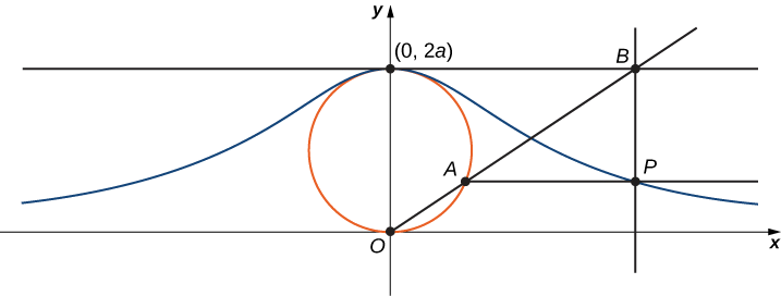
On the Figure $\PageIndex{13}$ label the following points, lengths, and the angle:

a. $C$ is the point on the $x$-axis with the same $x$-coordinate as $A$.

b. $x$ is the $x$-coordinate of $P$, and $y$ is the $y$-coordinate of $P$.

c. $E$ is the point $(0,a)$.

d. $F$ is the point on the line segment $OA$ such that the line segment $EF$ is perpendicular to the line segment $OA$.

e. $b$ is the distance from $O$ to $F$.

f. $c$ is the distance from $F$ to $A$.

g. $d$ is the distance from $O$ to $C$.

h. $θ$ is the measure of angle $∠COA$.

The goal of this project is to parameterize the witch using $θ$ as a parameter. To do this, write equations for $x$ and $y$ in terms of only $θ$.

2. Show that $d=\dfrac{2a}{\sin θ}$.

3. Note that $x=d\cos θ$. Show that $x=2a\cot θ$. When you do this, you will have parameterized the $x$-coordinate of the curve with respect to $θ$. If you can get a similar equation for $y$, you will have parameterized the curve.

4. In terms of $θ$, what is the angle $∠EOA$?

5. Show that $b+c=2a\cos\left(\frac{π}{2}−θ\right)$.

6. Show that $y=2a\cos\left(\frac{π}{2}−θ\right)\sin θ$.

7. Show that $y=2a\sin^2θ$. You have now parameterized the $y$-coordinate of the curve with respect to $θ$.

8. Conclude that a parameterization of the given witch curve is

$$x=2a\cot θ, \quad y=2a \sin^2θ, \quad\text{for }−∞<θ<∞.$$

9. Use your parameterization to show that the given witch curve is the graph of the function $f(x)=\dfrac{8a^3}{x^2+4a^2}$

Travels with My Ant: The Curate and Prolate Cycloids

Earlier in this section, we looked at the parametric equations for a cycloid, which is the path a point on the edge of a wheel traces as the wheel rolls along a straight path. In this project we look at two different variations of the cycloid, called the curtate and prolate cycloids.

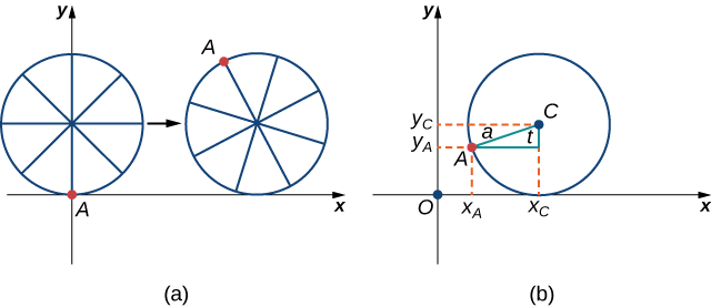
First, let’s revisit the derivation of the parametric equations for a cycloid. Recall that we considered a tenacious ant trying to get home by hanging onto the edge of a bicycle tire. We have assumed the ant climbed onto the tire at the very edge, where the tire touches the ground. As the wheel rolls, the ant moves with the edge of the tire (Figure $\PageIndex{14}$).

As we have discussed, we have a lot of flexibility when parameterizing a curve. In this case we let our parameter t represent the angle the tire has rotated through. Looking at (Figure $\PageIndex{12}$), we see that after the tire has rotated through an angle of $t$, the position of the center of the wheel, $C=(x_C,y_C)$, is given by

$x_C=at$ and $y_C=a$.

Furthermore, letting $A=(x_A,y_A)$ denote the position of the ant, we note that

$x_C−x_A=a\sin t$ and $y_C−y_A=a \cos t$

Then

$$x_A=x_C−a\sin t=at−a\sin t=a(t−\sin t)$$

$$y_A=y_C−a\cos t=a−a\cos t=a(1−\cos t).$$

(a) has a circle with point A on the circle at the origin. The circle has “spokes,” with point A being at the end of one of these spokes. The circle appears to be traveling to the right on the x-axis, with point A being up above the x-axis in a second image of the circle drawn slightly to the right. (b) has a circle in the first quadrant with center C. It touches the x-axis at $x_c$. A point, A is drawn on the circle and a right triangle is made from this point and point C. The hypotenuse is marked a and the angle at C between A and $x_c$ is marked t. Lines are drawn to give the x and y values of A as $x_A$ and $y_A$, respectively. Similarly, a line is drawn to give the y value of C as $y_C$.

Figure $\PageIndex{14}$: (a) The ant clings to the edge of the bicycle tire as the tire rolls along the ground. (b) Using geometry to determine the position of the ant after the tire has rotated through an angle of $t$.

Note that these are the same parametric representations we had before, but we have now assigned a physical meaning to the parametric variable $t$.

After a while the ant is getting dizzy from going round and round on the edge of the tire. So he climbs up one of the spokes toward the center of the wheel. By climbing toward the center of the wheel, the ant has changed his path of motion. The new path has less up-and-down motion and is called a curtate cycloid Figure $\PageIndex{15}$. As shown in the figure, we let b denote the distance along the spoke from the center of the wheel to the ant. As before, we let t represent the angle the tire has rotated through. Additionally, we let $C=(x_C,y_C)$ represent the position of the center of the wheel and $A=(x_A,y_A)$ represent the position of the ant.

(a) has a circle with “spokes,” where point A is in the middle of one of these spokes. The circle is tangent to the x-axis at the origin. The circle appears to be traveling to the right on the x-axis, with point A being higher up in a second image of the circle drawn slightly to the right. (b) shows the curve that point A would trace out, as the circle travels to the right. It is vaguely sinusoidal. (c) has a circle in the first quadrant with center C. It touches the x-axis at $x_c$. A point, A is drawn inside the circle and a right triangle is made from this point and point C. The hypotenuse is marked b, the angle at C between A and xc is marked t, and the distance from C to $x_c$ is marked a. Lines are drawn to give the x and y values of A as $x_A$ and $y_A$, respectively. Similarly, a line is drawn to give the y value of C as $y_C$.

Figure $\PageIndex{15}$: (a) The ant climbs up one of the spokes toward the center of the wheel. (b) The ant’s path of motion after he climbs closer to the center of the wheel. This is called a curtate cycloid. (c) The new setup, now that the ant has moved closer to the center of the wheel.

1. What is the position of the center of the wheel after the tire has rotated through an angle of $t$?

2. Use geometry to find expressions for $x_C−x_A$ and for $y_C−y_A$.

3. On the basis of your answers to parts 1 and 2, what are the parametric equations representing the curtate cycloid?

Once the ant’s head clears, he realizes that the bicyclist has made a turn, and is now traveling away from his home. So he drops off the bicycle tire and looks around. Fortunately, there is a set of train tracks nearby, headed back in the right direction. So the ant heads over to the train tracks to wait. After a while, a train goes by, heading in the right direction, and he manages to jump up and just catch the edge of the train wheel (without getting squished!).

The ant is still worried about getting dizzy, but the train wheel is slippery and has no spokes to climb, so he decides to just hang on to the edge of the wheel and hope for the best. Now, train wheels have a flange to keep the wheel running on the tracks. So, in this case, since the ant is hanging on to the very edge of the flange, the distance from the center of the wheel to the ant is actually greater than the radius of the wheel Figure $\PageIndex{16}$.

The setup here is essentially the same as when the ant climbed up the spoke on the bicycle wheel. We let b denote the distance from the center of the wheel to the ant, and we let t represent the angle the tire has rotated through. Additionally, we let $C=(x_C,y_C)$ represent the position of the center of the wheel and $A=(x_A,y_A)$ represent the position of the ant (Figure $\PageIndex{14}$).

When the distance from the center of the wheel to the ant is greater than the radius of the wheel, his path of motion is called a prolate cycloid. A graph of a prolate cycloid is shown in the figure. (a) has a circle and a point A that is outside the circle on the y-axis (below the origin). The circle is tangent to the x-axis at the origin. The circle appears to be traveling to the right on the x-axis, with point A being above the x-axis in a second image of the circle drawn slightly to the right. Figure b has a circle in the first quadrant with center C. It touches the x-axis at $x_c$. A point, A is drawn outside the circle and a right triangle is made from this point and point C. The hypotenuse is marked b, the angle at C between A and $x_c$ is marked t, and the distance from C to $x_c$ is marked a. Lines are drawn to give the x and y values of A as $x_A$and $y_A$, respectively. Similarly, a line is drawn to give the y value of C as $y_C$. Figure c shows the curve that point A would trace out, as the circle travels to the right. It is vaguely sinusoidal with an extra loop at the bottom once per revolution.

Figure $\PageIndex{16}$: (a) The ant is hanging onto the flange of the train wheel. (b) The new setup, now that the ant has jumped onto the train wheel. (c) The ant travels along a prolate cycloid.

4. Using the same approach you used in parts 1– 3, find the parametric equations for the path of motion of the ant.

5. What do you notice about your Solution to part 3 and your Solution to part 4?

Notice that the ant is actually traveling backward at times (the “loops” in the graph), even though the train continues to move forward. He is probably going to be really dizzy by the time he gets home!

Key Concepts

• Parametric equations provide a convenient way to describe a curve. A parameter can represent time or some other meaningful quantity.
• It is often possible to eliminate the parameter in a parameterized curve to obtain a function or relation describing that curve.
• There is always more than one way to parameterize a curve.
• Parametric equations can describe complicated curves that are difficult or perhaps impossible to describe using rectangular coordinates.

Glossary

Cycloid

The curve traced by a point on the rim of a circular wheel as the wheel rolls along a straight line without slippage

Cusp

A pointed end or part where two curves meet

Orientation

The direction that a point moves on a graph as the parameter increases

Parameter

An independent variable that both $x$ and $y$ depend on in a parametric curve; usually represented by the variable $t$

Parametric curve

The graph of the parametric equations $x(t)$ and $y(t)$ over an interval $a≤t≤b$ combined with the equations

Parametric equations

The equations $x=x(t)$ and $y=y(t)$ that define a parametric curve

Parameterization of a curve

Rewriting the equation of a curve defined by a function $y=f(x)$ as parametric equations

Contributors and Attributions

• Gilbert Strang (MIT) and Edwin “Jed” Herman (Harvey Mudd) with many contributing authors. This content by OpenStax is licensed with a CC-BY-SA-NC 4.0 license. Download for free at http://cnx.org.