
6.3: Separable Equations
- Page ID
- 212057

\( \newcommand{\vecs}[1]{\overset { \scriptstyle \rightharpoonup} {\mathbf{#1}} } \)
\( \newcommand{\vecd}[1]{\overset{-\!-\!\rightharpoonup}{\vphantom{a}\smash {#1}}} \)
\( \newcommand{\dsum}{\displaystyle\sum\limits} \)
\( \newcommand{\dint}{\displaystyle\int\limits} \)
\( \newcommand{\dlim}{\displaystyle\lim\limits} \)
\( \newcommand{\id}{\mathrm{id}}\) \( \newcommand{\Span}{\mathrm{span}}\)
( \newcommand{\kernel}{\mathrm{null}\,}\) \( \newcommand{\range}{\mathrm{range}\,}\)
\( \newcommand{\RealPart}{\mathrm{Re}}\) \( \newcommand{\ImaginaryPart}{\mathrm{Im}}\)
\( \newcommand{\Argument}{\mathrm{Arg}}\) \( \newcommand{\norm}[1]{\| #1 \|}\)
\( \newcommand{\inner}[2]{\langle #1, #2 \rangle}\)
\( \newcommand{\Span}{\mathrm{span}}\)
\( \newcommand{\id}{\mathrm{id}}\)
\( \newcommand{\Span}{\mathrm{span}}\)
\( \newcommand{\kernel}{\mathrm{null}\,}\)
\( \newcommand{\range}{\mathrm{range}\,}\)
\( \newcommand{\RealPart}{\mathrm{Re}}\)
\( \newcommand{\ImaginaryPart}{\mathrm{Im}}\)
\( \newcommand{\Argument}{\mathrm{Arg}}\)
\( \newcommand{\norm}[1]{\| #1 \|}\)
\( \newcommand{\inner}[2]{\langle #1, #2 \rangle}\)
\( \newcommand{\Span}{\mathrm{span}}\) \( \newcommand{\AA}{\unicode[.8,0]{x212B}}\)
\( \newcommand{\vectorA}[1]{\vec{#1}} % arrow\)
\( \newcommand{\vectorAt}[1]{\vec{\text{#1}}} % arrow\)
\( \newcommand{\vectorB}[1]{\overset { \scriptstyle \rightharpoonup} {\mathbf{#1}} } \)
\( \newcommand{\vectorC}[1]{\textbf{#1}} \)
\( \newcommand{\vectorD}[1]{\overrightarrow{#1}} \)
\( \newcommand{\vectorDt}[1]{\overrightarrow{\text{#1}}} \)
\( \newcommand{\vectE}[1]{\overset{-\!-\!\rightharpoonup}{\vphantom{a}\smash{\mathbf {#1}}}} \)
\( \newcommand{\vecs}[1]{\overset { \scriptstyle \rightharpoonup} {\mathbf{#1}} } \)
\(\newcommand{\longvect}{\overrightarrow}\)
\( \newcommand{\vecd}[1]{\overset{-\!-\!\rightharpoonup}{\vphantom{a}\smash {#1}}} \)
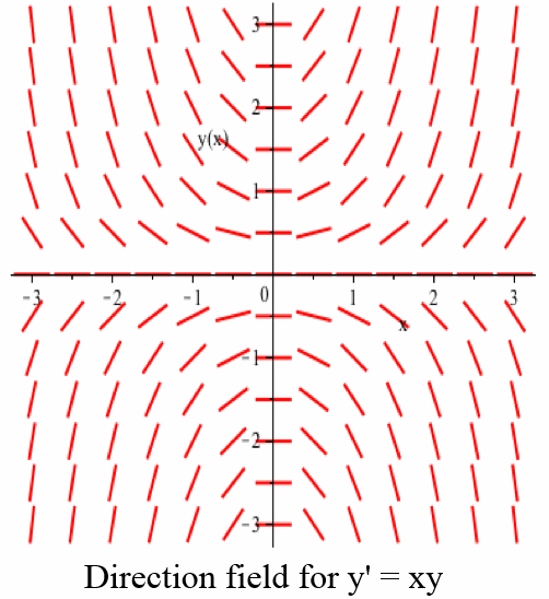
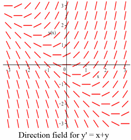
\(\newcommand{\avec}{\mathbf a}\) \(\newcommand{\bvec}{\mathbf b}\) \(\newcommand{\cvec}{\mathbf c}\) \(\newcommand{\dvec}{\mathbf d}\) \(\newcommand{\dtil}{\widetilde{\mathbf d}}\) \(\newcommand{\evec}{\mathbf e}\) \(\newcommand{\fvec}{\mathbf f}\) \(\newcommand{\nvec}{\mathbf n}\) \(\newcommand{\pvec}{\mathbf p}\) \(\newcommand{\qvec}{\mathbf q}\) \(\newcommand{\svec}{\mathbf s}\) \(\newcommand{\tvec}{\mathbf t}\) \(\newcommand{\uvec}{\mathbf u}\) \(\newcommand{\vvec}{\mathbf v}\) \(\newcommand{\wvec}{\mathbf w}\) \(\newcommand{\xvec}{\mathbf x}\) \(\newcommand{\yvec}{\mathbf y}\) \(\newcommand{\zvec}{\mathbf z}\) \(\newcommand{\rvec}{\mathbf r}\) \(\newcommand{\mvec}{\mathbf m}\) \(\newcommand{\zerovec}{\mathbf 0}\) \(\newcommand{\onevec}{\mathbf 1}\) \(\newcommand{\real}{\mathbb R}\) \(\newcommand{\twovec}[2]{\left[\begin{array}{r}#1 \\ #2 \end{array}\right]}\) \(\newcommand{\ctwovec}[2]{\left[\begin{array}{c}#1 \\ #2 \end{array}\right]}\) \(\newcommand{\threevec}[3]{\left[\begin{array}{r}#1 \\ #2 \\ #3 \end{array}\right]}\) \(\newcommand{\cthreevec}[3]{\left[\begin{array}{c}#1 \\ #2 \\ #3 \end{array}\right]}\) \(\newcommand{\fourvec}[4]{\left[\begin{array}{r}#1 \\ #2 \\ #3 \\ #4 \end{array}\right]}\) \(\newcommand{\cfourvec}[4]{\left[\begin{array}{c}#1 \\ #2 \\ #3 \\ #4 \end{array}\right]}\) \(\newcommand{\fivevec}[5]{\left[\begin{array}{r}#1 \\ #2 \\ #3 \\ #4 \\ #5 \\ \end{array}\right]}\) \(\newcommand{\cfivevec}[5]{\left[\begin{array}{c}#1 \\ #2 \\ #3 \\ #4 \\ #5 \\ \end{array}\right]}\) \(\newcommand{\mattwo}[4]{\left[\begin{array}{rr}#1 \amp #2 \\ #3 \amp #4 \\ \end{array}\right]}\) \(\newcommand{\laspan}[1]{\text{Span}\{#1\}}\) \(\newcommand{\bcal}{\cal B}\) \(\newcommand{\ccal}{\cal C}\) \(\newcommand{\scal}{\cal S}\) \(\newcommand{\wcal}{\cal W}\) \(\newcommand{\ecal}{\cal E}\) \(\newcommand{\coords}[2]{\left\{#1\right\}_{#2}}\) \(\newcommand{\gray}[1]{\color{gray}{#1}}\) \(\newcommand{\lgray}[1]{\color{lightgray}{#1}}\) \(\newcommand{\rank}{\operatorname{rank}}\) \(\newcommand{\row}{\text{Row}}\) \(\newcommand{\col}{\text{Col}}\) \(\renewcommand{\row}{\text{Row}}\) \(\newcommand{\nul}{\text{Nul}}\) \(\newcommand{\var}{\text{Var}}\) \(\newcommand{\corr}{\text{corr}}\) \(\newcommand{\len}[1]{\left|#1\right|}\) \(\newcommand{\bbar}{\overline{\bvec}}\) \(\newcommand{\bhat}{\widehat{\bvec}}\) \(\newcommand{\bperp}{\bvec^\perp}\) \(\newcommand{\xhat}{\widehat{\xvec}}\) \(\newcommand{\vhat}{\widehat{\vvec}}\) \(\newcommand{\uhat}{\widehat{\uvec}}\) \(\newcommand{\what}{\widehat{\wvec}}\) \(\newcommand{\Sighat}{\widehat{\Sigma}}\) \(\newcommand{\lt}{<}\) \(\newcommand{\gt}{>}\) \(\newcommand{\amp}{&}\) \(\definecolor{fillinmathshade}{gray}{0.9}\)So far, we have only learned how to solve ODEs of the form \(y' = f(x)\) (which you already knew how to solve), where \(y'\) depended only on \(x\) and the slopes of the line segments of a corresponding direction field did not depend on the \(y\)-coordinate of the location of the line segment. In many situations, however, \(y'\) depends on both \(x\) and \(y\), for example, \(y' = xy\):
or \(y' = x + y\):
In Example 2 of Section 2.9, we considered the problem of finding a tangent line to the circle \(x^2+y^2 = 25\) at the point \((3,4)\). You can solve this problem geometrically. Or you can solve the equation for \(y\) to get \(y = \sqrt{25-x^2}\) and then compute \(\displaystyle \frac{dy}{dx}\). Or you can implicitly differentiate the equation \(x^2+y^2=25\), keeping in mind that \(y\) is a function of \(x\):\[x^2+y^2 = 25 \ \Rightarrow \ 2x + 2y \cdot \frac{dy}{dx} = 0 \ \Rightarrow \ 2y \cdot \frac{dy}{dx} = -2x \ \Rightarrow \ \frac{dy}{dx} = -\frac{x}{y}\nonumber\]The result is a differential equation (although we didn't call it that in Section 2.9) and putting \(x=3\) and \(y=4\) into the right side of that ODE yields \(\displaystyle \frac{dy}{dx} = -\frac34\), which gives us the slope of the line tangent to the circle at the point \((3,4)\).
What if we start with \(\displaystyle \frac{dy}{dx} = -\frac{x}{y}\) and try to solve this ODE? It is not of the form \(y' = f(x)\), but we can try to solve it by beginning to reverse the steps in the implicit differentiation process above:\[\frac{dy}{dx} = -\frac{x}{y} \quad \Rightarrow \quad y \cdot \frac{dy}{dx} = -x\nonumber\]Each side of this new ODE is a function of \(x\) because \(y\) and \(\displaystyle \frac{dy}{dx}\) are functions of \(x\), so we can integrate both sides of this equation to get:\[\int y \cdot \frac{dy}{dx} \, dx = \int -x \, dx \ \Rightarrow \ \frac12 y^2 + C_1 = -\frac12 x^2 + C_2\nonumber\](Each indefinite integral yields a constant, but these are not necessarily equal.)
The integration on the left-hand side of this equation uses the fact that:\[\frac{d}{dx}\left[\frac12 y^2\right] = \frac12 \cdot 2 y \cdot \frac{dy}{dx} = y \cdot \frac{dy}{dx}\nonumber\]but this is the same result as if we had “cancelled” the \(dx\) in the original left-hand integral:\[\int y \cdot \frac{dy}{dx} \, dx = \int y \, dy = \frac12 y^2 + C_1\nonumber\]so in our first steps above we could have instead rewritten the ODE using differentials:\[\frac{dy}{dx} = -\frac{x}{y} \ \Rightarrow \ y \cdot \frac{dy}{dx} = -x \ \Rightarrow y\, dy = -x \, dx \ \Rightarrow \int y \, dy = \int -x \, dx\nonumber\]and then integrated both sides. (We will follow this procedure as we solve similar ODEs from now on.) We can now move both constants of integration to the same side of the equation:\[\frac12 y^2 = -\frac12 x^2 + \left[C_2-C_1\right] \ \Rightarrow \ \frac12 y^2 = -\frac12 x^2 + K\nonumber\]where \(K\) is another arbitrary constant. Because we can always move the left-hand constant to the right side of the equation and combine it with the right-hand constant, in the future we will use a single constant on the right side when integrating both sides of the differential equation.
At this stage we can write:\[\frac12 y^2 = -\frac12 x^2 + K \ \Rightarrow \ y^2 = -x^2 + 2K \ \Rightarrow x^2+y^2 = C\nonumber\]where \(C\) is yet another arbitrary constant. We recognize this as an equation for a circle centered at the origin and we call a solution of this type an implicit solution to the ODE because we have not explicitly solved for \(y\). If we know our solution curve passes through \((3,4)\), we can put this information into our solution equation to get:\[3^2+4^2 = C \ \Rightarrow \ C = 25 \ \Rightarrow \ x^2+y^2 = 25\nonumber\]Solving for \(y\), we get \(\displaystyle y = \sqrt{25-x^2}\), an explicit solution to the ODE. (We first get \(\displaystyle y = \pm\sqrt{25-x^2}\) but knowing that \(y(3) = 4\) tells us to use the \(+\) symbol rather than the \(-\) symbol.)
Separable Equations
In the ODE we solved above, we were able to “separate” the variables so that only \(y\) appeared on one side and only \(x\) appeared on the other, allowing us to integrate each side separately to solve the ODE.
A differential equation is called separable if we can separate the variables algebraically so that the equation has the form:\[g(y) \cdot y' = f(x)\nonumber\]
If possible, separate the variables in each ODE by writing the given differential equation in the form \(g(y)\cdot y' = f(x)\):
- \(\displaystyle y' = xy\)
- \(\displaystyle x y' = \frac{y+1}{x}\)
- \(\displaystyle y' = \frac{1 + \sin(x)}{y^2 + y}\)
- \(\displaystyle y' = y\)
- \(y' = x+y\)
Solution
- Divide each side of \(y' = xy\) by \(y\) (to do so we must assume \(y \neq 0\)) to get \(\displaystyle \frac{1}{y}\cdot y' = x\) so \(\displaystyle g(y) = \frac{1}{y}\) and \(f(x) = x\).
- Divide each side by \(x(y+1)\) (to do so we must assume \(x \neq 0\) and \(y \neq -1\)) to get \(\displaystyle \frac{1}{y+1} \cdot y' = \frac{1}{x^2}\) so \(\displaystyle g(y) = \frac{1}{y+1}\) and \(\displaystyle f(x) = \frac{1}{x^2}\).
- Multiply each side by \(y^2 + y\) to get \(\displaystyle \left(y^2 + y\right)\cdot y' = 1 + \sin(x)\) so \(g(y) = y^2 + y\) and \(f(x) = 1+\sin(x)\).
- Divide each side by \(y\) (to do so we must assume \(y \neq 0\)) to get \(\displaystyle \frac{1}{y} \cdot y' = 1\) so \(\displaystyle g(y) = \frac{1}{y}\) and \(f(x) = 1\).
- We cannot write this ODE in the form \(g(y)\cdot y' = f(x)\).
The first four ODEs are separable, but the last one is not.
If possible, separate the variables in each ODE by writing the given differential equation in the form \(g(y)\cdot y' = f(x)\):
- \(y' = x^3(y - 5)\)
- \(\displaystyle y' = \frac{3}{2x + x\cdot\sin(y+2)}\)
- Answer
-
- If \(y \neq 5\), divide the ODE \(y' = x^3(y-5)\) by \(y-5\) to get \(\displaystyle \frac{1}{y-5} \cdot \frac{dy}{dx} = x^3\) so \(g(y) = \displaystyle \frac{1}{y-5}\) and \(f(x) = x^3\).
- Factor \(x\) out of the denominator on the right-hand side and multiply both sides of the ODE by \(2+\sin(y+2)\) to get:\[\frac{dy}{dx} = \frac{3}{x\left[2+\sin(y+2)\right]} \quad \Rightarrow \quad \left[2+\sin(y+2)\right]\cdot \frac{dy}{dx} = \frac{3}{x}\nonumber\]so \(g(y) = 2+\sin(y+2)\) and \(\displaystyle f(x) = \frac{3}{x}\).
Solving Separable ODEs
To solve a separable differential equation, we will follow the steps outlined above when solving \(\displaystyle \frac{dy}{dx} = -\frac{x}{y}\):
- Use algebra to separate the variables in the ODE: \(g(y) \cdot y' = f(x)\)
- Put into an equivalent form using differentials: \(g(y) \, dy = f(x) \, dx\)
- Integrate each side of the equation: \(\displaystyle \int g(y) \, dy = \int f(x) \, dx\)
- Find antiderivatives, if possible: \(G(y) = F(x) + C\)
- If given an initial condition \(\left(x_0,y_0\right)\), find \(C\): \(C = G\left(y_0\right)-F\left(x_0\right)\)
- If possible, solve explicitly for \(y\).
Find the general solution of \(\displaystyle \frac{1}{x} \cdot y' = \frac{x}{2y}\).
Solution
Multiply each side by \(2xy\) to get \(2y \cdot y' = x^2\), so the ODE is separable and we can translate it into differential form:\[2y\cdot \frac{dy}{dx} = x^2 \quad \Rightarrow \quad 2y \, dy = x^2\, dx\nonumber\]Integrating each side, we get:\[\int 2y\, dy = \int x^2\, dx \quad \Rightarrow \quad y^2 = \frac13 x^3 + C\nonumber\]which is an implicit form of the general solution. Solving for \(y\), we get:\[y = \pm \sqrt{\frac13 x^3 + C}\nonumber\]which is an explicit form of the general solution.
Find the solution of \(\displaystyle y' = \frac{6x + 1}{2y}\) that satisfies \(y(2) = 3\).
Solution
We can rewrite this ODE as \(2y\cdot y' = 6x + 1\), so it is separable. Next rewrite using differentials:\[2y\cdot \frac{dy}{dx} = 6x + 1 \quad \Rightarrow \quad 2y\, dy = \left( 6x + 1 \right)\, dx\nonumber\]and then integrate each side:\[\int 2y \, dy = \int \left(6x + 1\right)\, dx \quad \Rightarrow \quad y^2 = 3x^2 + x + C\nonumber\]Putting \(x = 2\) and \(y = 3\) into the general solution \(y^2 = 3x^2 + x + C\):\[3^2 = 3\cdot 2^2 + 2 + C \quad \Rightarrow \quad 9 = 12 + 2 + C \quad \Rightarrow \quad C = -5\nonumber\](In an initial value problem, it is often easier to solve for \(C\) immediately after finding the antiderivatives.) So \(y^2 = 3x^2 + x - 5 \quad \Rightarrow \quad y = \pm\sqrt{3x^2 + x - 5}\). Because \(y(2) = 3\), we need the \(+\) value of the square root: \(y = \sqrt{3x^2 + x - 5}\).
Find the general solution of \(\displaystyle y' = \frac{1 - \sin(x)}{3y^2}\) and then find the solution that passes through \((0,2)\).
- Answer
-
Multiply both sides of the ODE by \(3y^2\) to get:\[3y^2 \cdot \frac{dy}{dx} = 1 - \sin(x) \quad \Rightarrow \quad 3y^2 \, dy = \left[1-\sin(x)\right] \, dx\nonumber\]and integrate:\[\int 3y^2 \, dy = \int \left[1-\sin(x)\right] \, dx \quad \Rightarrow \quad y^3 = x +\cos(x) + C\nonumber\]This is an implicit form of the general solution; an explicit general solution is \(\displaystyle y = \sqrt[3]{x +\cos(x) + C}\).
Using the initial condition \(y(0)=2\) with the implicit form of the general solution:\[2^3 = 0 + \cos(0) + C \ \Rightarrow 8 = 1 + C \quad \Rightarrow \quad C = 7\nonumber\]so the solution to the IVP is \(\displaystyle y = \sqrt[3]{x +\cos(x) + 7}\).
Sometimes algebra is the hardest part of solving an ODE, and often logarithms crop up when solving separable equations.
Solve \(x\cdot y' = y + 3\).
Solution
To write the ODE in the form \(g(y)\cdot y' = f(x)\) we can divide by \(x\) and by \(y+3\) (so we must assume that \(x \neq 0\) and \(y \neq -3\)):\[x\cdot \frac{dy}{dx} = y + 3 \ \Rightarrow \ \frac{1}{y+3} \, \frac{dy}{dx} = \frac{1}{x} \ \Rightarrow \frac{1}{y+3} \, dy = \frac{1}{x} \, dx\nonumber\]Now integrate both sides:\[\int \frac{1}{y+3} \, dy = \int \frac{1}{x} \, dx \quad \Rightarrow \quad \ln\left(\left|y+3\right|\right) = \ln\left(\left|x\right|\right) + C\nonumber\]which is an implicit form of the general solution. To explicitly solve for \(y\), recall that \(\displaystyle e^{\ln\left( a \right)} = a\) so:\[e^{\ln\left(\left|y+3\right|\right)} = e^{\ln\left(\left|x\right|\right) + C} = e^{\ln\left(\left|x\right|\right)} \cdot e^C \quad \Rightarrow \quad \left|y+3\right| = e^C \cdot \left|x\right|\nonumber\]Removing the absolute value signs we get:\[y+3 = \pm e^C \cdot x \quad \Rightarrow \quad y = \pm e^C x - 3 \quad \Rightarrow \quad y = Ax-3\nonumber\]where \(A\) is any nonzero constant. In the first step above, we had to assume that \(y \neq -3\). You can check that the constant function \(y = -3\) is also a solution to the ODE: \(x \cdot \left[-3\right]' = -3 + 3\). So \(y = Ax-3\) is a solution of the ODE even when \(A = 0\), and the general solution of the ODE is \(y = Ax-3\) for any value of \(A\).
Study the direction field for \(x\cdot y' = y+3\) shown below:

What do you notice about its behavior near the lines \(x = 0\) and \(y=-3\)?
The domain of any particular solution of the form \(y = Ax-3\) is either \((-\infty,0)\) or \((0,\infty)\), which is related to the assumption that \(x \neq 0\) in our solution. Putting \(x=0\) into the original ODE yields \(0 = y + 3 \Rightarrow y -3\), so the only solution for which \(x=0\) is the single point \((0,-3)\) rather than a function defined on an open interval.
Existence and Uniqueness
In Section 6.2, we saw that any IVP of the form \(y' = f(x)\), \(y\left(x_0\right) = y_0\) had a unique solution: that is, at least one solution to the IVP exists, and this solution is the only possible solution. Unfortunately, for other types of IVPs things can be more complicated.
The ODE \(y^2+\left(y'\right)^2 = -1\) has no solution, no matter what initial value condition we might specify. (Can you see why?) The ODE \(y^2+\left(y'\right)^2 = 0\) has only one solution (the constant solution \(y=0\)) so the IVP \(y^2+\left(y'\right)^2 = 0\), \(y(0) = 0\) has one unique solution, but the IVP \(y^2+\left(y'\right)^2 = 0\), \(y(0) = 5\) has none.
Even separable equations can behave in unexpected ways. Consider the IVP \(\displaystyle y' = 3 y^{\frac23}\), \(y(0) = 0\). The ODE is separable (if \(y\neq 0\)):\[\frac{dy}{dx} = 3y^{\frac23} \quad \Rightarrow \quad \frac13 y^{-\frac23} \frac{dy}{dx} = 1 \quad \Rightarrow \quad \frac13 y^{-\frac23}\, dy = dx\nonumber\]Integrating both sides:\[\int \frac13 y^{-\frac23}\, dy = \int 1 \, dx \quad \Rightarrow \quad y^{\frac13} = x + C \quad \Rightarrow \quad y = (x+C)^3\nonumber\]Using the initial condition, \(0 = y(0) = (0+C)^3 = C^3 \ \Rightarrow \ C = 0\) so \(y = x^3\) solves the IVP. But we had to assume that \(y \neq 0\); checking the constant function \(y = 0\), \(\left[0\right]' = 3\cdot 0^{\frac23}\) and \(y(0) = 0\), so \(y(x) = 0\) also satisfies the IVP, giving the IVP two solutions: \(y(x) = 0\) and \(y(x) = x^3\).
(In a course on differential equations, you will learn about a theorem that specifies restrictions on a first-order IVP that will guarantee a unique solution.)
Problems
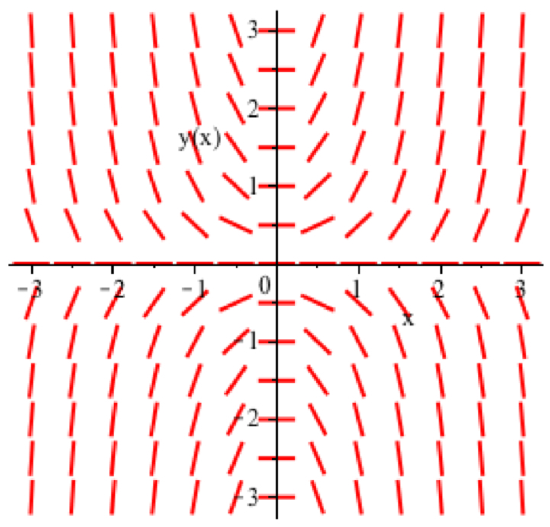
- The direction field of the separable ODE \(y' = 2xy\) appears below:
Sketch solutions of the ODE that satisfy the initial conditions \(y(0) = 1\), \(y(0) = -1\) and \(y(1) = 2\). - The direction field of the separable ODE \(\displaystyle y' = x/y\) appears below:

Sketch solutions of the ODE that satisfy the initial conditions \(y(0) = 1\), \(y(0) = -1\) and \(y(1) = 2\).
In Problems 3–10, solve the separable ODE.
- \(y' = 2xy\)
- \(\displaystyle y' = \frac{x}{y}\)
- \(\left(1 + x^2\right)\cdot y' = 3\)
- \(xy' = y + 3\)
- \(y' \cdot \cos(x) = e^y\)
- \(y' = x^2 y + 3y\)
- \(y' = 4y\)
- \(y' = 5(2 - y)\)
In Problems 11–18, solve the separable ODEs subject to the given initial conditions.
- \(y' = 2xy\) for \(y(0) = 3\), \(y(0) = 5\) and \(y(1) = 2\).
- \(\displaystyle y' = \frac{x}{y}\) for \(y(0) = 3\), \(y(0) = 5\) and \(y(1) = 2\).
- \(y' = 3y\) for \(y(0) = 4\), \(y(0) = 7\) and \(y(1) = 3\).
- \(y' = -2y\) for \(y(0) = 4\), \(y(0) = 7\) and \(y(1) = 3\).
- \(y' = 5(2 - y)\) for \(y(0) = 5\) and \(y(0) = -3\).
- \(y' = 7(1 - y)\) for \(y(0) = 4\) and \(y(0) = -2\).
- \(\left(1 + x^2\right)\cdot y' = 3\) for \(y(1) = 4\) and \(y(0) = 2\).
- \(xy' = y + 3\) for \(y(1) = 20\).
- For \(xy' = y + 3\), can \(y(0) = 2\)?
- Find all solutions to the IVP \(y' = \sqrt[3]{y}\), \(y(0) = 0\).