7.1: One-to-One Functions

You’ve seen that some equations have only one solution (for example, \(5 - 2x = 3\) and \(x^3 = 8\)), while some have two solutions (\(x^2 + 3 = 7\)) and some even have an infinite number of solutions (\(\sin(x) = 0.8\)). The graphs of \(y = 5 - 2x\), \(y = x^3\), \(y = x^2 + 3\) and \(y = \sin(x)\) and the solutions of the equations mentioned above appear below:

Functions \(f\) for which equations of the form \(f(x) = k\) have at most one solution for each value of \(k\) (that is, each outcome \(k\) comes from only one input \(x\)) arise often in applications and possess a number of useful mathematical properties. This brief section focuses on those functions and examines some of their properties.

Example \(\PageIndex{1}\)

1. \(f(x) = 0\) for \(f(x) = x(x - 4)\)
2. \(g(x) = 3\) for \(g\) given in the table below:

   \(x\)	0	1	2	3	4	5
   \(g(x)\)	5	7	3	5	0	7

3. \(h(x) = 4\) for \(h\) given by the graph below:
   
4. \(f(x) = k\) for \(f(x) = e^x\).

Solution

1. Two: \(x(4 - x) = 0 \Rightarrow x = 0\) or \(x = 4\).
2. One: \(g(x) = 3\) only if \(x = 2\).
3. Two: \(h(x) = 4\) if \(x \approx 1.2\) or if \(x \approx 4\).
4. If \(k > 0\), it has one solution: \(x = \ln(k)\). If \(k \leq 0\), it has no solutions.

Practice \(\PageIndex{1}\)

How many solutions does each equation have?

1. \(f(x) = 4\) for \(f(x) = x(4 - x)\)
2. \(g(x) = 7\) for \(g\) given by the table from Example \(\PageIndex{1}\).
3. \(H(x) = 3\) for \(H\) given by the graph below:
   
4. \(f(x) = 5\) for \(f(x) = \ln(x)\)

Answer

1. One: solve \(x(4 - x) = 4\) to get \(x = 2\).
2. Two: \(x = 1\) and \(x = 5\).
3. One: \(x \approx 3.5\).
4. One: solve \(5 = \ln(x)\) to get \(x = e^5 \approx 148.4\).

Horizontal Line Test

You should be familiar with the Vertical Line Test, a graphical tool you can use to help determine whether or not a curve in the \(xy\)-plane is the graph of a function. (If not, review Section 0.3.) A similar geometrical test leads to the definition of a one-to-one function and provides a tool for helping to determine when a function is one-to-one.

Horizontal Line Test (Definition of One-to-One)

A function is one-to-one if each horizontal line intersects the graph of the function at most once.

Equivalently, a function \(y = f(x)\) is one-to-one if two distinct \(x\)-values always produce two distinct \(y\)-values: that is, \(a \neq b \Rightarrow f(a) \neq f(b)\). This immediately tells us that every strictly increasing function is one-to-one, and that every strictly decreasing function is one-to-one. (Why?)

For any function, if we know an input value we can calculate the output, but an output may arise from any of several different inputs. With a one-to-one function, each output comes from only one input.

Example \(\PageIndex{2}\)

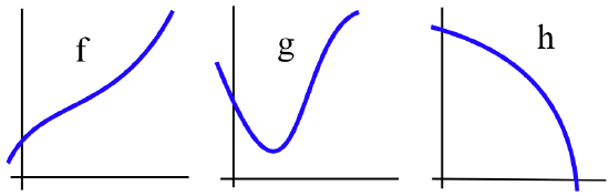
1. Which functions in the figure below are one-to-one?
   
2. Which functions in the table below are one-to-one?

   \(x\)	\(f(x)\)	\(g(x)\)	\(h(x)\)
   0	5	7	2
   1	2	3	-1
   2	3	0	5
   3	5	1	4
   4	0	6	3
   5	1	3	0

Solution

1. In the figure, \(f\) and \(h\) are one-to-one; \(g\) fails the Horizontal Line Test, so \(g\) is not one-to-one.
2. In the table, \(h\) is one-to-one, while \(f\) and \(g\) are not one-to-one because \(f(0) = f(3)\) and \(g(1) = g(5)\).

Practice \(\PageIndex{2}\)

1. Which functions graphed below are one-to-one?
   
2. Which functions in the table below are one-to-one?

   \(x\)	\(f(x)\)	\(g(x)\)	\(h(x)\)
   0	4	2	-2
   1	2	3	5
   2	-2	0	1
   3	5	4	14
   4	3	6	3
   5	1	7	1

Answer

1. Only \(g\) is one-to-one; \(f\) and \(h\) fail the Horizontal Line Test.
2. Both \(f\) and \(g\) are one-to-one; \(h\) is not, because \(h(2)=h(5)\).

Example \(\PageIndex{3}\)

Let \(f(x) = 2x + 1\):

Find the values of \(x\) so that:

1. \(f(x) = 9\) and
2. \(f(x) = a\) and then
3. solve \(f(y) = x\) for \(y\).

Solution

1. \(9 = f(x) = 2x + 1 \Rightarrow 8 = 2x  \Rightarrow x = \frac82 = 4\)
2. \(a = 2x + 1\) \(\Rightarrow 2x = a - 1 \Rightarrow x = \frac{a - 1}{2}\)
3. \(\displaystyle x = f(y) = 2y + 1 \Rightarrow 2y = x - 1\) so \(\displaystyle y = \frac{x - 1}{2}\). Notice that this new function reverses the operations of \(f(x)\), applied in reverse order: \(f(x)\) multiplies \(x\) by \(2\), then adds \(1\); the new function subtracts \(1\), then divides by \(2\).

Practice \(\PageIndex{3}\)

Let \(g(x) = 3x - 5\). Find the values of \(x\) so that:

1. \(g(x) = 7\) and
2. \(g(x) = b\) and then
3. solve \(g(y) = x\) for \(y\).

Answer

1. \(3x - 5 = 7 \Rightarrow 3x=12 \Rightarrow x = 4\)
2. \(\displaystyle 3x - 5 = a \Rightarrow 3x = a + 5 \Rightarrow x = \frac{a+5}{3}\)
3. \(\displaystyle f(x) = 3x - 5 \Rightarrow f(y) = 3y-5\) so \(\displaystyle f(y) = x \Rightarrow 3y-5 = x \Rightarrow 3y=x+5 \Rightarrow y = \frac{x+5}{3}\)

Practice \(\PageIndex{4}\)

Show that exponential growth, for example \(f(x) = e^{3x}\), and exponential decay, for example \(g(x) = e^{-2x}\), are both one-to-one.

Answer

If \(f(x) = e^{kx}\) where \(k>0\) then \(f'(x) = k\cdot e^{kx} > 0\) so \(f(x)\) is strictly increasing, hence one-to-one. If \(g(x) = e^{rx}\) where \(r<0\) then \(g'(x) = r\cdot e^{rx} < 0\) so \(g(x)\) is strictly decreasing, hence one-to-one.

Problems

In Problems 1–4, explain why each given function is (or is not) one-to-one.

1. \(f(x) = 3x - 5\), \(y = 3 - x\), \(g(x)\) given by the table below:

   \(x\)	\(g(x)\)
   0	3
   1	4
   2	5
   3	2
   4	4

   and \(h(x)\) given by the graph below:
   
2. \(\displaystyle f(x) = \frac{x}{4}\), \(y = x^2 + 3\), \(g(x)\) given by the table below:

   \(x\)	\(g(x)\)
   0	3
   1	2
   2	0
   3	-2
   4	1

   and \(h(x)\) given by the graph below:
   
3. \(\displaystyle f(x) = \sin(x)\), \(y = e^x - 2\), \(g(x)\) given by the table below:

   \(x\)	\(g(x)\)
   0	-1
   1	5
   2	3
   3	1
   4	0

   and \(h(x)\) given by the graph below:
   
4. \(\displaystyle f(x) = 17\), \(y = x^3-1\), \(g(x)\) given by the table below:

   \(x\)	\(g(x)\)
   0	2
   1	5
   2	4
   3	1
   4	2

   and \(h(x)\) given by the graph below:
   
5. Is the relation between people and Social Security numbers a function? A one-to-one function?
6. Is the relation between people and phone numbers a function? If so, is it one-to-one?
7. What would it mean if the scores on a calculus test were one-to-one?
8. The relation given below represents “\(y\) is married to \(x\)”:

   \(x\)	A	B	C	D
   \(y\)	P	Q	P	R

   1. Is this relation a function?
   2. Is it one-to-one?
   3. Is P breaking the law?
   4. Is A breaking the law?
9. In how many places can a one-to-one function touch the \(x\)-axis?
10. Can a continuous one-to-one function have the values given below? Explain.

    \(x\)	1	3	5
    \(f(x)\)	2	7	3

11. The graph of \(f(x) = x - 2\cdot\lfloor x \rfloor\) for \(-2 \leq x \leq 3\) appears below:
    
    1. Is \(f\) a one-to-one function?
    2. Is \(f\) an increasing function?
    3. Is \(f\) a decreasing function?
12. Is every linear function \(L(x) = ax + b\) one-to-one? If not, which linear functions are one-to-one?
13. Show that \(f(x) = \ln(x)\) is one-to-one for \(x > 0\).
14. Show that \(g(x) = e^x\) is one-to-one.
15. The table below gives an encoding rule for a six-letter alphabet:

    a	b	c	d	e	f
    d	c	f	e	b	a

    1. Is the encoding rule a function?
    2. Is the encoding rule one-to-one?
    3. Encode the word “bad.”
    4. Create a table for decoding the encoded letters and use it to decode your answer to part (c).
    5. A graph of the encoding rule appears below:
       
       Create a graph of the decoding rule.
    6. Compare the encoding and decoding graphs.
16. The table below gives an encoding rule for a six-letter alphabet:

    a	b	c	d	e	f
    b	d	b	b	a	c

    1. Is the encoding rule a function?
    2. Is the encoding rule one-to-one?
    3. Encode the word “bad.”
    4. Create a table for decoding the encoded letters and use it to decode your answer to part (c).
    5. Create a graph of the encoding rule.
    6. Create a graph of the decoding rule.
    7. Compare the encoding and decoding graphs.
17. The table below gives an encoding rule for a six-letter alphabet:

    a	b	c	d	e	f
    d	f	e	a	c	b

    1. Is the encoding rule a function?
    2. Is the encoding rule one-to-one?
    3. Encode the word “bad.”
    4. Create a table for decoding the encoded letters and use it to decode your answer to part (c).
    5. Create a graph of the encoding rule.
    6. Create a graph of the decoding rule.
    7. Compare the encoding and decoding graphs.
    8. What happens if you encode a word, then encode the encoded word? For example, \(\mbox{encode}\left(\mbox{encode}\left(\mbox{“bad”}\right)\right) = \mbox{?}\)
18. The table below gives an encoding rule for a six-letter alphabet:

    a	b	c	d	e	f
    e	a	f	c	b	d

    1. Is the encoding rule a function?
    2. Is the encoding rule one-to-one?
    3. Encode the word “bad.”
    4. Create a table for decoding the encoded letters and use it to decode your answer to part (c).
    5. Create a graph of the encoding rule.
    6. Create a graph of the decoding rule.
    7. Compare the encoding and decoding graphs.
    8. What happens if you apply this encoding rule three times in succession? For example: \(\mbox{encode}\left(\mbox{encode}\left(\mbox{encode}\left(\mbox{“bad”}\right)\right)\right) = \mbox{?}\)