
7.2: Inverse Functions
- Page ID
- 212064

\( \newcommand{\vecs}[1]{\overset { \scriptstyle \rightharpoonup} {\mathbf{#1}} } \)
\( \newcommand{\vecd}[1]{\overset{-\!-\!\rightharpoonup}{\vphantom{a}\smash {#1}}} \)
\( \newcommand{\dsum}{\displaystyle\sum\limits} \)
\( \newcommand{\dint}{\displaystyle\int\limits} \)
\( \newcommand{\dlim}{\displaystyle\lim\limits} \)
\( \newcommand{\id}{\mathrm{id}}\) \( \newcommand{\Span}{\mathrm{span}}\)
( \newcommand{\kernel}{\mathrm{null}\,}\) \( \newcommand{\range}{\mathrm{range}\,}\)
\( \newcommand{\RealPart}{\mathrm{Re}}\) \( \newcommand{\ImaginaryPart}{\mathrm{Im}}\)
\( \newcommand{\Argument}{\mathrm{Arg}}\) \( \newcommand{\norm}[1]{\| #1 \|}\)
\( \newcommand{\inner}[2]{\langle #1, #2 \rangle}\)
\( \newcommand{\Span}{\mathrm{span}}\)
\( \newcommand{\id}{\mathrm{id}}\)
\( \newcommand{\Span}{\mathrm{span}}\)
\( \newcommand{\kernel}{\mathrm{null}\,}\)
\( \newcommand{\range}{\mathrm{range}\,}\)
\( \newcommand{\RealPart}{\mathrm{Re}}\)
\( \newcommand{\ImaginaryPart}{\mathrm{Im}}\)
\( \newcommand{\Argument}{\mathrm{Arg}}\)
\( \newcommand{\norm}[1]{\| #1 \|}\)
\( \newcommand{\inner}[2]{\langle #1, #2 \rangle}\)
\( \newcommand{\Span}{\mathrm{span}}\) \( \newcommand{\AA}{\unicode[.8,0]{x212B}}\)
\( \newcommand{\vectorA}[1]{\vec{#1}} % arrow\)
\( \newcommand{\vectorAt}[1]{\vec{\text{#1}}} % arrow\)
\( \newcommand{\vectorB}[1]{\overset { \scriptstyle \rightharpoonup} {\mathbf{#1}} } \)
\( \newcommand{\vectorC}[1]{\textbf{#1}} \)
\( \newcommand{\vectorD}[1]{\overrightarrow{#1}} \)
\( \newcommand{\vectorDt}[1]{\overrightarrow{\text{#1}}} \)
\( \newcommand{\vectE}[1]{\overset{-\!-\!\rightharpoonup}{\vphantom{a}\smash{\mathbf {#1}}}} \)
\( \newcommand{\vecs}[1]{\overset { \scriptstyle \rightharpoonup} {\mathbf{#1}} } \)
\(\newcommand{\longvect}{\overrightarrow}\)
\( \newcommand{\vecd}[1]{\overset{-\!-\!\rightharpoonup}{\vphantom{a}\smash {#1}}} \)
\(\newcommand{\avec}{\mathbf a}\) \(\newcommand{\bvec}{\mathbf b}\) \(\newcommand{\cvec}{\mathbf c}\) \(\newcommand{\dvec}{\mathbf d}\) \(\newcommand{\dtil}{\widetilde{\mathbf d}}\) \(\newcommand{\evec}{\mathbf e}\) \(\newcommand{\fvec}{\mathbf f}\) \(\newcommand{\nvec}{\mathbf n}\) \(\newcommand{\pvec}{\mathbf p}\) \(\newcommand{\qvec}{\mathbf q}\) \(\newcommand{\svec}{\mathbf s}\) \(\newcommand{\tvec}{\mathbf t}\) \(\newcommand{\uvec}{\mathbf u}\) \(\newcommand{\vvec}{\mathbf v}\) \(\newcommand{\wvec}{\mathbf w}\) \(\newcommand{\xvec}{\mathbf x}\) \(\newcommand{\yvec}{\mathbf y}\) \(\newcommand{\zvec}{\mathbf z}\) \(\newcommand{\rvec}{\mathbf r}\) \(\newcommand{\mvec}{\mathbf m}\) \(\newcommand{\zerovec}{\mathbf 0}\) \(\newcommand{\onevec}{\mathbf 1}\) \(\newcommand{\real}{\mathbb R}\) \(\newcommand{\twovec}[2]{\left[\begin{array}{r}#1 \\ #2 \end{array}\right]}\) \(\newcommand{\ctwovec}[2]{\left[\begin{array}{c}#1 \\ #2 \end{array}\right]}\) \(\newcommand{\threevec}[3]{\left[\begin{array}{r}#1 \\ #2 \\ #3 \end{array}\right]}\) \(\newcommand{\cthreevec}[3]{\left[\begin{array}{c}#1 \\ #2 \\ #3 \end{array}\right]}\) \(\newcommand{\fourvec}[4]{\left[\begin{array}{r}#1 \\ #2 \\ #3 \\ #4 \end{array}\right]}\) \(\newcommand{\cfourvec}[4]{\left[\begin{array}{c}#1 \\ #2 \\ #3 \\ #4 \end{array}\right]}\) \(\newcommand{\fivevec}[5]{\left[\begin{array}{r}#1 \\ #2 \\ #3 \\ #4 \\ #5 \\ \end{array}\right]}\) \(\newcommand{\cfivevec}[5]{\left[\begin{array}{c}#1 \\ #2 \\ #3 \\ #4 \\ #5 \\ \end{array}\right]}\) \(\newcommand{\mattwo}[4]{\left[\begin{array}{rr}#1 \amp #2 \\ #3 \amp #4 \\ \end{array}\right]}\) \(\newcommand{\laspan}[1]{\text{Span}\{#1\}}\) \(\newcommand{\bcal}{\cal B}\) \(\newcommand{\ccal}{\cal C}\) \(\newcommand{\scal}{\cal S}\) \(\newcommand{\wcal}{\cal W}\) \(\newcommand{\ecal}{\cal E}\) \(\newcommand{\coords}[2]{\left\{#1\right\}_{#2}}\) \(\newcommand{\gray}[1]{\color{gray}{#1}}\) \(\newcommand{\lgray}[1]{\color{lightgray}{#1}}\) \(\newcommand{\rank}{\operatorname{rank}}\) \(\newcommand{\row}{\text{Row}}\) \(\newcommand{\col}{\text{Col}}\) \(\renewcommand{\row}{\text{Row}}\) \(\newcommand{\nul}{\text{Nul}}\) \(\newcommand{\var}{\text{Var}}\) \(\newcommand{\corr}{\text{corr}}\) \(\newcommand{\len}[1]{\left|#1\right|}\) \(\newcommand{\bbar}{\overline{\bvec}}\) \(\newcommand{\bhat}{\widehat{\bvec}}\) \(\newcommand{\bperp}{\bvec^\perp}\) \(\newcommand{\xhat}{\widehat{\xvec}}\) \(\newcommand{\vhat}{\widehat{\vvec}}\) \(\newcommand{\uhat}{\widehat{\uvec}}\) \(\newcommand{\what}{\widehat{\wvec}}\) \(\newcommand{\Sighat}{\widehat{\Sigma}}\) \(\newcommand{\lt}{<}\) \(\newcommand{\gt}{>}\) \(\newcommand{\amp}{&}\) \(\definecolor{fillinmathshade}{gray}{0.9}\)If \(f\) is any one-to-one function then equations of the form \(f(x) = k\) have (at most) a single solution. Such functions can be uniquely “undone”: if \(f\) is a one-to-one function, then there is another function \(g\) that “undoes” the effect of \(f\), so that \(g\left( f(x) \right) = x\). When \(g\) and \(f\) are composed in this manner, \(g\) retrieves the original input of \(f\):

We call this function \(g\) that “undoes” the effect of \(f\) the inverse function of \(f\) or simply the inverse of \(f\).
If \(f\) is a function that encodes a message, then the inverse of \(f\) is the function that decodes an encoded message to retrieve the original message. The functions \(e^x\) and \(\ln(x)\) “undo” the effects of each other:\[\ln\left( e^x \right) = x \quad \mbox{and} \quad e^{\ln(x)} = x \ (\mbox{for } x > 0)\nonumber\]so the functions \(e^x\) and \(\ln(x)\) are inverses of each other.
This section will examine some of the properties of inverse functions and explain how to find the inverse of a function given by a table of data, a graph or a formula.
If \(f\) and \(g\) are functions that satisfy both \(g\left( f(x) \right) = x\) and \(f\left( g(y) \right) = y\) for all \(x\) in the domain of \(f\) and all \(y\) in the domain of \(g\), then \(g\) is the inverse of \(f\), \(f\) is the inverse of \(g\), and \(f\) and \(g\) are a pair of inverse functions.
We often write the inverse function of \(f\) as \(f^{-1}\) (pronounced “eff inverse”) but you must be very careful: \(f^{-1}\) does not mean \(\displaystyle \frac{1}{f}\).
The values of a function \(f\) appear in the table below:
| \(x\) | \(f(x)\) |
|---|---|
| \(0\) | \(3\) |
| \(1\) | \(2\) |
| \(2\) | \(0\) |
| \(3\) | \(1\) |
Evaluate \(\displaystyle f^{-1}(0)\) and \(\displaystyle f^{-1}(1)\).
Solution
For every \(x\), \(\displaystyle f^{-1}\left( f(x) \right) = x\) so the value of \(f^{-1}(0)\) is the solution \(x\) of the equation \(f(x) = 0\). The value we want is \(x = 2\), and we can check that \(\displaystyle f^{-1}(0) = f^{-1}\left( f(2) \right) = 2\).
The value of \(f^{-1}(1)\) is the solution \(x\) of the equation \(f(x) = 1\), which is \(x = 3\), and we can check that \(\displaystyle f^{-1}(1) = f^{-1}\left( f(3) \right) = 3\).
Similarly, \(f^{-1}(2) = 1\) and \(f^{-1}(3) = 0\). These results appear in the table below:
| \(x\) | \(f^{-1}(x)\) |
|---|---|
| \(0\) | \(2\) |
| \(1\) | \(3\) |
| \(2\) | \(1\) |
| \(3\) | \(0\) |
You should notice that if the ordered pair \((a,b)\) is in the table for \(f\), then the reversed pair \((b,a)\) is in the table for \(f^{-1}\).
The values of the function \(g\) appear in the table below:
| \(x\) | \(g(x)\) |
|---|---|
| \(0\) | \(2\) |
| \(1\) | \(1\) |
| \(2\) | \(3\) |
| \(3\) | \(4\) |
| \(4\) | \(0\) |
Create a table of values for \(g^{-1}\).
- Answer
-
\(x\) \(g^{-1}(x)\) \(0\) \(4\) \(1\) \(1\) \(2\) \(0\) \(3\) \(2\) \(4\) \(3\)
The method of interchanging the coordinates of a point on the graph (or in a table of values) of \(f\) to get a point on the graph (or in a table of values) of \(f^{-1}\) provides an efficient way to graph \(f^{-1}\).
If the point \((a,b)\) is on the graph of \(f\), then the point \((b,a)\) is on the graph of \(f^{-1}\).
Proof
If \((a,b)\) is on the graph of \(f\), then \(b = f(a)\), so \(f^{-1}(b) = f^{-1}\left( f(a) \right)\). By definition, \(f^{-1}\left( f(a) \right) =a\), so \(f^{-1}(b) = a\), which tells us that \((b,a)\) is on the graph of \(f^{-1}\).
Graphically, when you interchange the coordinates of a point \((a,b)\) to get a new point \((b,a)\), the old point and the new point are symmetric about the line \(y = x\). If you put a spot of wet ink at the point \((a,b)\) on a piece of graph paper:

and fold the paper along the line \(y = x\), a new spot of ink will appear at the point \((b,a)\). The figures below demonstrate another graphical method for finding the location of the point \((b,a)\):

Draw the line \(y=x\) along with a line of slope \(-1\) that passes through the given point \(P\) (above left), then measure the distance from \(P\) to the line \(y=x\) and move that same distance on the other side of \(y=x\) (above center), and plot the new point \(Q\) at that location.
The graphs of \(f\) and \(f^{-1}\) are symmetric about the line \(y = x\).
A graph of \(f\) appears below:

Sketch a graph of \(f^{-1}\).
Solution
Imagine the graph of \(f\) is drawn with wet ink and fold the \(xy\)-plane along the line \(y = x\). When you unfold the plane, the new graph is \(f^{-1}\):

You could also proceed point by point: Pick several points \((a,b)\) on the graph of \(f\) and plot the symmetric points \((b,a)\), then use the new \((b,a)\) points as a guide for sketching the graph of \(f^{-1}\).
A graph of \(g\) appears below:

Sketch a graph of \(g^{-1}\). What happens to points on the graph of \(g\) that lie on the line \(y = x\)?
- Answer
-
FIGURE
If a point lies on the line \(y=x\), it must have the form \((a,a)\) so that \(g(a) = a \Rightarrow a = g^{-1}(a)\): the point \((a,a)\) is also on the graph of \(g^{-1}\).
Finding a Formula for \(f^{-1}(x)\)
When you have a table of values for \(f\), you can create a table of values for \(f^{-1}\) by interchanging the values of \(x\) and \(y\) in the table for \(f\) (as in Example \(\PageIndex{1}\)). When you have a graph of \(f\), you can sketch a graph of \(f^{-1}\) by reflecting the graph of \(f\) about the line \(y = x\) (as in Example \(\PageIndex{2}\)). When you have a formula for \(f\), you can try to find a formula for \(f^{-1}\).
The steps for wrapping a gift are:
- put the gift in a box,
- cover the box with paper and
- attach a ribbon.
What are the steps for opening the gift — the inverse of the wrapping operation?
Solution
- Remove the ribbon (undo step 3),
- remove the paper (undo step 2) and
- remove the gift from the box (undo step 1
(Then show happiness and gratitude.)
The reason for the preceding trivial example is to point out that the first unwrapping step undoes the last wrapping step, the second unwrapping step undoes the second-to-last wrapping step … and the last unwrapping step undoes the first wrapping step. This pattern holds for functions and their inverses too.
The steps to evaluate \(f(x) = 9x + 6\) are:
- multiply the input by \(9\) and
- add \(6\) to the result.
Write the steps, in words, for the inverse of this function, and then translate the verbal steps for the inverse into a formula for the inverse function.
Solution
- Subtract \(6\), undoing (2), and
- divide by \(9\), undoing (1):
\[x \quad \longrightarrow \quad x - 6 \quad \longrightarrow \quad \frac{x-6}{9}\nonumber\]so \(\displaystyle f^{-1}(x) = \frac{x - 6}{9}\) provides a formula for the inverse function.
If \((x, y)\) is a point on the graph of \(f\), we know that \((y, x)\) is on the graph of \(f^{-1}\), so interchanging the roles of \(x\) and \(y\) in the formula for \(f\) should lead us to a formula for \(f^{-1}\). Applying this idea to the function \(f(x) = 9x + 6\) from the previous Example, we swap \(x\) and \(y\) in the formula \(y = 9x + 6\) to get \(\displaystyle x = 9y + 6 \Rightarrow x - 6 = 9y \Rightarrow y = \frac{x-6}{9}\), yielding the formula \(\displaystyle f^{-1}(x) = \frac{x - 6}{9}\) as in Example 4.
The following algorithm provides a general “recipe” for finding a formula for an inverse function:
- Start with a formula for \(f\): \(y = f(x)\).
- Interchange the roles of \(x\) and \(y\): \(x = f(y)\).
- Solve \(x = f(y)\) for \(y\).
- The resulting formula for \(y\) is the inverse of \(f\): \(y = f^{-1}(x)\).
The “interchange” and “solve” steps in the algorithm effectively undo the original operations in reverse order.
Find formulas for the inverses \(f^{-1}(x)\) and \(g^{-1}(x)\) of \(\displaystyle f(x) = \frac{7x - 5}{4}\) and \(g(x) = 2e^{5x}\).
Solution
Starting with \(\displaystyle y = f(x) = \frac{7x - 5}{4}\) and interchanging the roles of \(x\) and \(y\) yields:\[x = \frac{7y - 5}{4} \ \Rightarrow \ 4x = 7y-5 \ \Rightarrow 4x+5 = 7y \ \Rightarrow \ y = \frac{4x+5}{7}\nonumber\]so \(\displaystyle f^{-1}(x) = \frac{4x+5}{7}\). Starting with \(y = g(x) = 2e^{5x}\) and interchanging the roles of \(x\) and \(y\) yields:\[x = 2e^{5y} \ \Rightarrow \ \frac{x}{2} = e^{5y} \ \Rightarrow \ \ln\left(\frac{x}{2}\right) = 5y \ \Rightarrow \ y = \frac15 \ln\left(\frac{x}{2}\right)\nonumber\]so \(\displaystyle g^{-1}(x) = \frac15 \ln\left(\frac{x}{2}\right)\).
Find formulas for the inverses \(f^{-1}(x)\), \(g^{-1}(x)\) and \(h^{-1}(x)\) of \(f(x) = 2x - 5\), \(\displaystyle g(x) = \frac{2x - 1}{x + 7}\) and \(h(x) = 2 + \ln(3x)\).
- Answer
-
- Swapping \(x\) and \(y\) in \(y = 2x-5\) yields \(\displaystyle x = 2y-5 \Rightarrow x+ 5 = 2y \Rightarrow y = \frac{x+5}{2}\) so \(\displaystyle f^{-1}(x) = \frac{x+5}{2}\).
- Swapping \(x\) and \(y\) in \(\displaystyle y = \frac{2x-1}{x+7}\): \(\displaystyle x = \frac{2y-1}{y+7} \Rightarrow xy+7x = 2y-1 \Rightarrow 7x+1 = 2y-xy \Rightarrow y = \frac{7x+1}{2-x}\) so \(\displaystyle g^{-1}(x) = \frac{7x+1}{2-x}\).
- Interchanging \(x\) and \(y\) in \(\displaystyle y = 2 + \ln(3x)\) yields \(\displaystyle x = 2+\ln(3y) \Rightarrow x-2 = \ln(3y) \Rightarrow e^{x-2} = 3y \Rightarrow y = \frac13 e^{x-2}\) so \(\displaystyle h^{-1}(x) = \frac13 e^{x-2}\).
Sometimes it is easy to “solve \(x = f(y)\) for \(y\),” but often it is not. When we try to find a formula for the inverse of \(y = f(x) = x + e^x\), the first step is easy: interchanging the roles of \(x\) and \(y\) yields \(x = y + e^y\). At this point, unfortunately, there is no way to algebraically solve the equation \(x = y + e^y\) explicitly for \(y\). The function \(y = x + e^x\) has an inverse function, but we cannot find an explicit formula for that inverse.
Which Functions Have Inverse Functions?
We have seen how to find the inverse function for some functions given by tables of values, by graphs and by formulas, but there are functions that do not have inverse functions. The only way a graph and its reflection about the line \(y = x\) can both be function graphs (so that \(f\) and \(f^{-1}\) are both functions) is if the graph of \(f\) passes both the Vertical Line Test (so that \(f\) is a function) and the Horizontal Line Test (so that the graph of \(f^{-1}\) passes the Vertical Line Test, verifying that \(f^{-1}\) is a function). This idea leads to the next theorem (stated without proof).
The function \(f\) has an inverse function if and only if \(f\) is one-to-one.
Two useful corollaries follow from this theorem.
If \(f\) is strictly increasing or strictly decreasing, then \(f\) has an inverse function.
If \(f'(x) > 0\) for all \(x\) or \(f'(x) < 0\) for all \(x\), then \(f\) has an inverse function.
Applying this last Corollary to \(f(x) = x + e^x\), we know that \(f'(x) = 1 + e^x > 0\) for all \(x\), so \(f\) must have an inverse (even though we can’t find an explicit formula for \(f^{-1}\)).
Slopes of Inverse Functions
When a function \(f\) has an inverse, the symmetry of the graphs of \(f\) and \(f^{-1}\) also provides us with information about slopes and derivatives.
Suppose the points \(P = (1,2)\) and \(Q = (3,6)\) are on the graph of a function \(f\).
- Sketch the line passing through \(P\) and \(Q\).
- Compute the slope of that line.
- Graph the reflected points \(P^*\) and \(Q^*\) on the graph of \(f^{-1}\).
- Sketch the line passing through \(P^*\) and \(Q^*\). Find the slope of the line through \(P^*\) and \(Q^*\).
Solution
- See the figure below.
- The slope through \(P\) and \(Q\) is \(\displaystyle m = \frac{6 - 2}{3 - 1} = \frac42 = 2\).
- The reflected points, obtained by interchanging the first and second coordinates of each point on the graph of \(f\), are \(P^* = (2,1)\) and \(Q^* = (6,3)\).
- See the figure below.
- The slope of the line though \(P^*\) and \(Q^*\) is \(\displaystyle \frac{3 - 1}{6 - 2} = \frac12\)

In the preceding Example, you may have noticed that:\[\mbox{slope of line through }P^* \mbox{ and }Q^* = \frac{1}{\mbox{slope of line through }P\mbox{ and }Q}\nonumber\]This was not a coincidence. In general, if \(P = (a,b)\) and \(Q = (x,y)\) are points on the graph of \(f\):

then the reflected points \(P^* = (b,a)\) and \(Q^* = (y,x)\) are on the graph of \(f^{-1}\) and:\[\mbox{slope of segment }P^*Q^* = \frac{1}{\mbox{slope of segment }PQ}\nonumber\]Because the slope of a tangent line is the limit of slopes of secant lines, a similar relationship holds between the slope of the tangent line to \(f\) at the point \((a,b)\) and slope of the tangent line to \(f^{-1}\) at the point \((b,a)\). If we let the point \(Q^*\) approach the point \(P^*\) along the graph of \(f^{-1}\):

then:
\begin{align*}\left(f^{-1}\right)'(b) &= \lim_{Q^* \to P^*} \, \left[\mbox{slope of segment }P^*Q^*\right] \\
&= \ \, \lim_{Q \to P} \ \frac{1}{\mbox{slope of segment }PQ} \ = \ \frac{1}{f'(a)}\end{align*}
This geometric idea leads to the following result:
If: \(b = f(a)\), \(f\) is differentiable at the point \((a,b)\) and \(f'(a) \neq 0\)
then: \(a = f^{-1}(b)\), \(f^{-1}\) is differentiable at the point \((b,a)\) and:\[\left(f^{-1}\right)'(b) = \frac{1}{f'(a)}\nonumber\]
The point \(\left(e^2, 2\right)\) is on the graph of \(f(x) = \ln(x)\) and \(\displaystyle f'(x) = \frac{1}{x} \Rightarrow f'\left(e^2\right) = \frac{1}{e^2}\). Let \(g\) be the inverse function of \(f\). Give one point on the graph of \(g\) and evaluate \(g'\) at that point.
Solution
The point \((2, e^2)\) is on the graph of \(g\) and:\[g'(2) = \frac{1}{f'(e^2)} = \frac{1}{\frac{1}{e^2}} = e^2\nonumber\]In fact, the inverse of \(f(x) = \ln(x)\) is the exponential function \(g(x) = e^x\) and we can check that \(g'(x) = e^x \Rightarrow g'(2) = e^2\).
In the table below, fill in the values of \(f^{-1}(x)\) and \(\left(f^{-1}\right)'(x)\) for \(x = 0\) and \(x = 1\):
| \(x\) | \(f(x)\) | \(f'(x)\) | \(f^{-1}(x)\) | \(\left(f^{-1}\right)'(x)\) |
|---|---|---|---|---|
| \(0\) | \(2\) | \(3\) | ||
| \(1\) | \(3\) | \(-2\) | ||
| \(2\) | \(1\) | \(-1\) | ||
| \(3\) | \(0\) | \(2\) |
Solution
\(f(3) = 0\), so \(f^{-1}(0) = 3\), while \(\displaystyle \left(f^{-1}\right)'(0) = \frac{1}{f'(3)} = \frac{1}{2}\); \(f(2) = 1\), so \(f^{-1}(1) = 2\) while \(\displaystyle \left(f^{-1}\right)'(1) = \frac{1}{f'(2)} = \frac{1}{-1} = -1\).
| \(x\) | \(f(x)\) | \(f'(x)\) | \(f^{-1}(x)\) | \(\left(f^{-1}\right)'(x)\) |
|---|---|---|---|---|
| \(0\) | \(2\) | \(3\) | \(3\) | \(0.5\) |
| \(1\) | \(3\) | \(-2\) | \(2\) | \(-1\) |
| \(1\) | \(3\) | \(-2\) | \(2\) | \(-1\) |
Fill in the missing values of \(f^{-1}(x)\) and \(\left(f^{-1}\right)'(x)\) in the table from Example for \(x = 2\) and \(x = 3\).
- Answer
-
\(f^{-1}(2) = 0\) and \(f^{-1}(3) = 1\) while \(\displaystyle \left(f^{-1}\right)'(2) = \frac{1}{f'(0)} = \frac{1}{3}\) and \(\displaystyle \left(f^{-1}\right)'(3) = \frac{1}{f'(1)} = \frac{1}{-2}\).
\(x\) \(f(x)\) \(f'(x)\) \(f^{-1}(x)\) \(\left(f^{-1}\right)'(x)\) \(2\) \(1\) \(-1\) \(0\) \(0.333\) \(3\) \(0\) \(2\) \(1\) \(-0.5\)
Problems
- Given the values of \(f\) and \(f'\) in the table below, compute the specified values of \(f^{-1}\) and \(\left(f^{-1}\right)'\).
\(x\) \(f(x)\) \(f'(x)\) \(f^{-1}(x)\) \(\left(f^{-1}\right)'(x)\) \(1\) \(3\) \(-3\) \(2\) \(1\) \(2\) \(3\) \(2\) \(3\) - Given the values of \(g\) and \(g'\) in the table below, compute the specified values of \(g^{-1}\) and \(\left(g^{-1}\right)'\).
\(x\) \(g(x)\) \(g'(x)\) \(g^{-1}(x)\) \(\left(g^{-1}\right)'(x)\) \(1\) \(2\) \(-2\) \(2\) \(1\) \(4\) \(3\) \(3\) \(2\) - Given the values of \(h\) and \(h'\) in the table below, compute the specified values of \(h^{-1}\) and \(\left(h^{-1}\right)'\).
\(x\) \(h(x)\) \(h'(x)\) \(h^{-1}(x)\) \(\left(h^{-1}\right)'(x)\) \(1\) \(2\) \(2\) \(2\) \(3\) \(-2\) \(3\) \(1\) \(0\) - Given the values of \(w\) and \(w'\) in the table below, compute the specified values of \(w^{-1}\) and \(\left(w^{-1}\right)'\).
\(x\) \(w(x)\) \(w'(x)\) \(w^{-1}(x)\) \(\left(w^{-1}\right)'(x)\) \(1\) \(1\) \(2\) \(2\) \(3\) \(0\) \(3\) \(2\) \(5\) - The figure below left shows a graph of \(f\). Sketch a graph of \(f^{-1}\).

- The figure above right shows a graph of \(g\). Sketch a graph of \(g^{-1}\).
- If the graphs of \(f\) and \(f^{-1}\) intersect at the point \((a ,b)\), how are \(a\) and \(b\) related?
- If the graph of \(f\) intersects the line \(y = x\) at \(x = a\), does the graph of \(f^{-1}\) intersect the line \(y = x\)? If so, where?
- The steps to evaluate the function \(\displaystyle f(x) = \frac{7x - 5}{4}\) are
- multiply by \(7\)
- subtract \(5\) and
- divide by \(4\).
- Find a formula for the inverse function of \(f(x) = 3x - 2\). Verify that \(f^{-1}\left( f(5) \right) = 5\) and \(f\left(f^{-1}(2)\right) = 2\).
- Find a formula for the inverse function of \(g(x) = 2x +1\). Verify that \(g^{-1}\left(g(1)\right) = 1\) and \(g\left(g^{-1}(7)\right) = 7\).
- Find a formula for the inverse of \(h(x) = 2e^{3x}\). Verify that \(h^{-1}\left(h(0)\right) = 0\).
- Find a formula for the inverse of \(w(x) = 5 + \ln(x)\). Verify that \(w^{-1}\left(w(1)\right) = 1\).
- If the graph of \(f\) goes through the point \((2, 5)\) and \(f'(2) = 3\), then the graph of \(f^{-1}\) goes through the point \(( \ \underline{\qquad} \, , \ \underline{\qquad} \ )\) and \(\left(f^{-1}\right)'(5)= \underline{\qquad}\).
- If the graph of \(f\) goes through the point \((1, 3)\) and \(f'(1) > 0\), then the graph of \(f^{-1}\) goes through the point \(( \ \underline{\qquad} \, , \ \underline{\qquad} \ )\). What can you say about the value of \(\left(f^{-1}\right)'(3)\)?
- If \(f(6) = 2\) and \(f'(6) < 0\), then the graph of \(f^{-1}\) goes through the point \(( \ \underline{\qquad} \, , \ \underline{\qquad} \ )\). What can you say about \(\left(f^{-1}\right)'(2)\)?
- If \(f '(x) > 0\) for all values of \(x\), what can you say about \(\left(f^{-1}\right)'(x)\)? What does this tell you about the graphs of \(f\) and \(f^{-1}\)?
- If \(f '(x) < 0\) for all values of \(x\), what can you say about \(\left(f^{-1}\right)'(x)\)? What does this tell you about the graphs of \(f\) and \(f^{-1}\)?
- Find a linear function \(f(x) = ax + b\) so the graphs of \(f\) and \(f^{-1}\) are parallel and do not intersect.
- Does \(f(x) = 3 + \sin(x)\) have an inverse function? Justify your answer.
- Does \(f(x) = 3x + \sin(x)\) have an inverse function? Justify your answer.
- For which positive integers \(n\) is \(f(x) = x^n\) one-to-one? Justify your answer.
- Some functions are their own inverses. For which four of these functions does \(f^{-1}(x) = f(x)\)?
- \(\displaystyle f(x) = \frac{1}{x}\)
- \(\displaystyle f(x) = \frac{x + 1}{x - 1}\)
- \(\displaystyle f(x) = \frac{3x - 5}{7x - 3}\)
- \(\displaystyle f(x) = \frac{ax + b}{cx - a}\)
- \(f(x) = x + a\) (\(a\neq 0\))
Reflections on Folding
The symmetry of the graphs of a function and its inverse about the line \(y = x\) make sketching a graph of the inverse function relatively easy if you have a graph of \(f\): fold your graph paper along the line \(y = x\) so the graph of \(f^{-1}\) is the “folded” image of \(f\). This simple idea of obtaining a new image of something by folding along a line can enable us to quickly “see” solutions to some otherwise difficult problems.
The minimization problem of finding the shortest path from town \(A\) to town \(B\) with an intermediate stop at a (straight) river, as depicted in below:
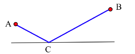
is moderately difficult to solve using derivatives (see Problem 11 in Section 3.5). Geometry allows us to solve the problem much more easily:

- obtain the point \(B^*\) by folding the image of \(B\) across the river line
- connect \(A\) and \(B^*\) with a line segment (the shortest path connecting \(A\) and \(B^*\))
- fold the \(C\)-to-\(B^*\) segment back across the river to obtain the \(A\)-to-\(C\)-to-\(B\) solution.
As an almost-free bonus, we see that — for the minimum path — the angle of incidence at the river equals the angle of reflection.
- Devise an algorithm using “folding” to locate the point at the bottom edge of the billiards table you should aim ball \(A\) in the figure below:

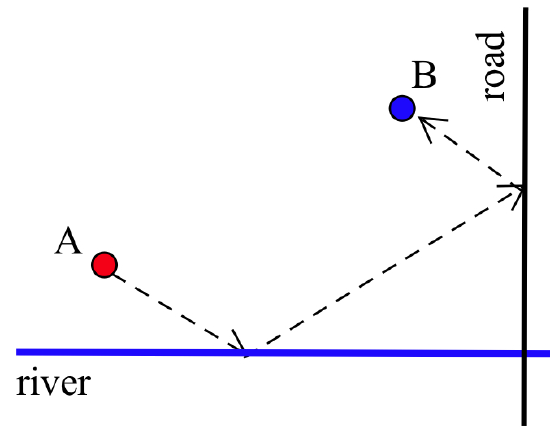
so that ball \(A\) will hit ball \(B\) after bouncing off the bottom edge of the table. (Assume that the angle of incidence equals the angle of reflection.) - Devise an algorithm using “folding” to sketch the shortest path in the figure below:
from town \(A\) to town \(B\) that includes a stop at the river and at the road. (One fold may not be enough.) - Devise an algorithm using “folding” to find where you should aim ball \(A\) at the bottom edge of the billiards table in the figure below so that ball \(A\) will hit ball \(B\) after bouncing off the bottom edge and the right edge of the table. (Assume that the angle of incidence equals the angle of reflection. Unfortunately, in a real-life game of billiards, the ball picks up a spin, called “English,” when it bounces off the first bank, so at the second bounce the angle of incidence does not equal the angle of reflection.)

The “folding” idea can even be useful if the path is not a straight line.
- The figure below shows the parabolic path of a thrown ball:

If the ball bounces off the tall vertical wall in this figure:
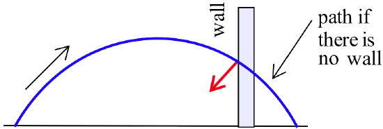
where will it hit the ground? (Assume that the angle of incidence equals the angle of reflection and that the ball does not lose energy during the bounce.)
Sometimes “unfolding” a problem is useful too.
- A spider and a fly are located at opposite corners of the cube as shown below:

Sketch the shortest path the spider can travel along the surface of the cube to reach the fly.