0.3: Functions and Their Graphs

Last updated
Save as PDF

Page ID: 209823

$ \newcommand{\vecs}[1]{\overset { \scriptstyle \rightharpoonup} {\mathbf{#1}} } $

$ \newcommand{\vecd}[1]{\overset{-\!-\!\rightharpoonup}{\vphantom{a}\smash {#1}}} $

$ \newcommand{\dsum}{\displaystyle\sum\limits} $

$ \newcommand{\dint}{\displaystyle\int\limits} $

$ \newcommand{\dlim}{\displaystyle\lim\limits} $

$ \newcommand{\id}{\mathrm{id}}$ $ \newcommand{\Span}{\mathrm{span}}$

( \newcommand{\kernel}{\mathrm{null}\,}\) $ \newcommand{\range}{\mathrm{range}\,}$

$ \newcommand{\RealPart}{\mathrm{Re}}$ $ \newcommand{\ImaginaryPart}{\mathrm{Im}}$

$ \newcommand{\Argument}{\mathrm{Arg}}$ $ \newcommand{\norm}[1]{\| #1 \|}$

$ \newcommand{\inner}[2]{\langle #1, #2 \rangle}$

$ \newcommand{\Span}{\mathrm{span}}$

$ \newcommand{\id}{\mathrm{id}}$

$ \newcommand{\Span}{\mathrm{span}}$

$ \newcommand{\kernel}{\mathrm{null}\,}$

$ \newcommand{\range}{\mathrm{range}\,}$

$ \newcommand{\RealPart}{\mathrm{Re}}$

$ \newcommand{\ImaginaryPart}{\mathrm{Im}}$

$ \newcommand{\Argument}{\mathrm{Arg}}$

$ \newcommand{\norm}[1]{\| #1 \|}$

$ \newcommand{\inner}[2]{\langle #1, #2 \rangle}$

$ \newcommand{\Span}{\mathrm{span}}$ $ \newcommand{\AA}{\unicode[.8,0]{x212B}}$

$ \newcommand{\vectorA}[1]{\vec{#1}} % arrow$

$ \newcommand{\vectorAt}[1]{\vec{\text{#1}}} % arrow$

$ \newcommand{\vectorB}[1]{\overset { \scriptstyle \rightharpoonup} {\mathbf{#1}} } $

$ \newcommand{\vectorC}[1]{\textbf{#1}} $

$ \newcommand{\vectorD}[1]{\overrightarrow{#1}} $

$ \newcommand{\vectorDt}[1]{\overrightarrow{\text{#1}}} $

$ \newcommand{\vectE}[1]{\overset{-\!-\!\rightharpoonup}{\vphantom{a}\smash{\mathbf {#1}}}} $

$ \newcommand{\vecs}[1]{\overset { \scriptstyle \rightharpoonup} {\mathbf{#1}} } $

$ \newcommand{\vecd}[1]{\overset{-\!-\!\rightharpoonup}{\vphantom{a}\smash {#1}}} $

$\newcommand{\avec}{\mathbf a}$ $\newcommand{\bvec}{\mathbf b}$ $\newcommand{\cvec}{\mathbf c}$ $\newcommand{\dvec}{\mathbf d}$ $\newcommand{\dtil}{\widetilde{\mathbf d}}$ $\newcommand{\evec}{\mathbf e}$ $\newcommand{\fvec}{\mathbf f}$ $\newcommand{\nvec}{\mathbf n}$ $\newcommand{\pvec}{\mathbf p}$ $\newcommand{\qvec}{\mathbf q}$ $\newcommand{\svec}{\mathbf s}$ $\newcommand{\tvec}{\mathbf t}$ $\newcommand{\uvec}{\mathbf u}$ $\newcommand{\vvec}{\mathbf v}$ $\newcommand{\wvec}{\mathbf w}$ $\newcommand{\xvec}{\mathbf x}$ $\newcommand{\yvec}{\mathbf y}$ $\newcommand{\zvec}{\mathbf z}$ $\newcommand{\rvec}{\mathbf r}$ $\newcommand{\mvec}{\mathbf m}$ $\newcommand{\zerovec}{\mathbf 0}$ $\newcommand{\onevec}{\mathbf 1}$ $\newcommand{\real}{\mathbb R}$ $\newcommand{\twovec}[2]{\left[\begin{array}{r}#1 \\ #2 \end{array}\right]}$ $\newcommand{\ctwovec}[2]{\left[\begin{array}{c}#1 \\ #2 \end{array}\right]}$ $\newcommand{\threevec}[3]{\left[\begin{array}{r}#1 \\ #2 \\ #3 \end{array}\right]}$ $\newcommand{\cthreevec}[3]{\left[\begin{array}{c}#1 \\ #2 \\ #3 \end{array}\right]}$ $\newcommand{\fourvec}[4]{\left[\begin{array}{r}#1 \\ #2 \\ #3 \\ #4 \end{array}\right]}$ $\newcommand{\cfourvec}[4]{\left[\begin{array}{c}#1 \\ #2 \\ #3 \\ #4 \end{array}\right]}$ $\newcommand{\fivevec}[5]{\left[\begin{array}{r}#1 \\ #2 \\ #3 \\ #4 \\ #5 \\ \end{array}\right]}$ $\newcommand{\cfivevec}[5]{\left[\begin{array}{c}#1 \\ #2 \\ #3 \\ #4 \\ #5 \\ \end{array}\right]}$ $\newcommand{\mattwo}[4]{\left[\begin{array}{rr}#1 \amp #2 \\ #3 \amp #4 \\ \end{array}\right]}$ $\newcommand{\laspan}[1]{\text{Span}\{#1\}}$ $\newcommand{\bcal}{\cal B}$ $\newcommand{\ccal}{\cal C}$ $\newcommand{\scal}{\cal S}$ $\newcommand{\wcal}{\cal W}$ $\newcommand{\ecal}{\cal E}$ $\newcommand{\coords}[2]{\left\{#1\right\}_{#2}}$ $\newcommand{\gray}[1]{\color{gray}{#1}}$ $\newcommand{\lgray}[1]{\color{lightgray}{#1}}$ $\newcommand{\rank}{\operatorname{rank}}$ $\newcommand{\row}{\text{Row}}$ $\newcommand{\col}{\text{Col}}$ $\renewcommand{\row}{\text{Row}}$ $\newcommand{\nul}{\text{Nul}}$ $\newcommand{\var}{\text{Var}}$ $\newcommand{\corr}{\text{corr}}$ $\newcommand{\len}[1]{\left|#1\right|}$ $\newcommand{\bbar}{\overline{\bvec}}$ $\newcommand{\bhat}{\widehat{\bvec}}$ $\newcommand{\bperp}{\bvec^\perp}$ $\newcommand{\xhat}{\widehat{\xvec}}$ $\newcommand{\vhat}{\widehat{\vvec}}$ $\newcommand{\uhat}{\widehat{\uvec}}$ $\newcommand{\what}{\widehat{\wvec}}$ $\newcommand{\Sighat}{\widehat{\Sigma}}$ $\newcommand{\lt}{<}$ $\newcommand{\gt}{>}$ $\newcommand{\amp}{&}$ $\definecolor{fillinmathshade}{gray}{0.9}$

When you prepared for calculus, you learned to manipulate functions by adding, subtracting, multiplying and dividing them, as well as evaluating functions of functions (composition). In calculus, we will continue to work with functions and their applications. We will create new functions by operating on old ones. We will gather information from the graphs of functions and from derived functions. We will find ways to describe the point-by-point behavior of functions as well as their behavior “close to” certain points and also over entire intervals. We will find tangent lines to graphs of functions and areas between graphs of functions. And, of course, we will see how these ideas can be used in a variety of fields.

This section and the next one review information and procedures you should already know about functions before we begin calculus.

What Is a Function?

Let’s begin with a (very) general definition of a function:

Definition

A function from a set $X$ to a set $Y$ is a rule for assigning to each element of the set $X$ a single element of the set $Y$. A function assigns a unique (exactly one) output element from the set $Y$ to each input element from the set $X$.

The rule that defines a function is often given in the form of an equation, but it could also be given in words or graphically or by a table of values. In practice, functions are given in all of these ways, and we will use all of them in this book.

In the definition of a function, the set $X$ of all inputs is called the domain of the function. The set $Y$ of all outputs produced from these inputs is called the range of the function. Two different inputs (elements in the domain) can be assigned to the same output (an element in the range) but one input cannot lead to two different outputs.

Most of the time we will work with functions whose domains and ranges are real numbers, but there are other types of functions all around us. Final grades for this course provide an example of a function. For each student, the instructor will assign a final grade based on some rule for evaluating that student’s performance. The domain of this function consists of all students registered for the course, and the range consists of grades (either letters like A, B, C, D, F, or numbers like 4.0, 3.7, 2.0, 1.7, 0.0). Two students can receive the same final grade, but only one grade can be assigned to each student.

Function Machines

Functions are abstract structures, but sometimes it is easier to think of them in a more concrete way. One such way is to imagine that a function is a special-purpose computer, a machine that accepts inputs, does something to those inputs according to a defining rule, and produces an output. The output is the value of the function associated with the given input value.

$Three side-by-side function machines, with input at the top and output at the bottom. The machine on the left has x going in and x^2 coming out; the middle machine has 5 going in and 25 coming out; the machine on the right has (c+3) going in and (c+3)^2 coming out.$

If the defining rule for a function $f$ is “multiply the input by itself,” $f(\mbox{input}) = (\mbox{input})(\mbox{input})$, then the figure and table in the margin show the results of putting the inputs $x$, $5$, $2.5$, $a$, $c + 3$ and $x + h$ into the machine $f$.

Input ($x$)	Output ($x^2$)
$x$	$x^2$
$a$	$a^2$
$2.5$	$6.25$
$x+h$	$(x+h)^2$

Practice $\PageIndex{1}$

If we have a function machine $g$ whose rule is “divide 3 by the input and add 1,” $g(x) = \frac{3}{x} + 1$, what outputs do we get from the inputs $x$, $5$, $a$, $c + 3$ and $x + h$? What happens if the input is $0$?

Answer

Create an input-output table using the function rule:

input	output
$x$	$\frac{3}{x}+1$
$5$	$\frac35 + 1 = 1.6$
$a$	$\frac{3}{a}+1$
$c+3$	$\frac{3}{c+3}+1$
$x+h$	$\frac{3}{x+h}+1$

If $x=0$, then $g(0) = \frac30 + 1$ is not defined (because of division by $0$).

You expect your calculator to behave as a function: each time you press the same sequence of keys (input) you expect to see the same display (output). In fact, if your calculator did not produce the same output each time, you would need a new calculator. (On many calculators there is a feature that does not produce the same output each time you use it. What is it?)

Functions Defined by Equations

If the domain of a function consists of a collection of real numbers (perhaps all real numbers) and the range is also a collection of real numbers, then the function is called a numerical function. We can give the rule for a numerical function in several ways, but usually write it as a formula. If the rule for a numerical function, $f$, is “the output is the input number multiplied by itself,” then we could write the rule as\[f(x) = x\cdot x = x^2\]The use of an “$x$” to represent the input is simply a matter of convenience and custom. We could also represent the same function by:

$f(a) = a^2$
$f(\#) = {\#}^2$ or
$f(\mbox{input}) = (\mbox{input})^2$.

For the function $f$ defined by $f(x) = x^2 - x$, we can see that:

$f(3) = 3^2 - 3 = 6$
$f(0.5) = (0.5)^2 - (0.5) = -0.25$
$f(-2) = (-2)^2 - (-2) = 6$

Notice that the two different inputs $3$ and $-2$ both lead to the output of $6$. That is allowable for a function.

We can also evaluate $f$ if the input contains variables. If we replace the “$x$” with something else in the notation “$f(x)$,” then we must replace the “$x$” with the same thing everywhere in the formula:

$f(c) = c^2 - c$
$f(a+1) = (a+1)^2 - (a+1) = (a^2 + 2a + 1) - (a + 1) = a^2 + a$
$f(x+h) = (x+h)^2 - (x+h) = (x^2+2xh+h^2) - (x+h)$

and, in general: $f(\mbox{input}) = (\mbox{input})^2 - (\mbox{input})$

For more complicated expressions, we can just proceed step-by-step:\begin{align*}
\frac{f(x+h) - f(x)}{h} &= \frac{\left((x+h)^2 - (x+h)\right) - \left(x^2- x\right)}{h}\\
&= \frac{\left((x^2+2xh+h^2) - (x+h)\right) - (x^2- x)}{h}\\
&= \frac{2xh + h^2 - h}{h} = \frac{h(2x + h - 1)}{h} = 2x + h - 1
\end{align*}

Practice $\PageIndex{2}$

For the function $g$ defined by $g(t) = t^2- 5t$, evaluate $g(1)$, $g(-2)$, $g(w+3)$, $g(x+h)$, $g(x+h) - g(x)$ and $\frac{g(x+h) - g(x)}{h}$.

Answer: $g(t) = t^2- 5t$
$g(1) = 1^2 - 5(1) = -4$
$g(-2) = (-2)^2 - 5(-2) = 14$
$g(w + 3) = (w + 3)^2 -5(w + 3) = w^2 + 6w + 9 - 5w - 15 = w^2 + w - 6$
$g(x + h) = (x + h)^2 - 5(x + h) = x^2 + 2xh + h^2 - 5x - 5h$
$g(x + h) - g(x) = (x^2 + 2xh + h^2- 5x - 5h ) - ( x^2 - 5x ) = 2xh + h^2- 5h$
$\displaystyle \frac{g(x + h) - g(x)}{h} = \frac{2xh + h^2 - 5h}{h} = 2x + h - 5$

Functions Defined by Graphs and Tables of Values

The graph of a numerical function $f$ consists of a plot of ordered pairs $(x,y)$ where $x$ is in the domain of $f$ and $y = f(x)$, such as the graph of $f(x) = \sin(x)$ for $-4 \leq x \leq 7$ below:

$A graph of y = sin(x) from x = -4 to x = 7.$

A table of values of a numerical function consists of a list of (some of) the ordered pairs $(x,y)$ where $y = f(x)$.

A function can be defined by a graph or by a table of values, and these types of definitions are common in applied fields. The outcome of an experiment will depend on the input, but the experimenter may not know the “rule” for predicting the outcome. In that case, the experimenter usually represents the function of interest as a table of measured outcome values versus input values, or as a graph of the outcomes versus the inputs. The table below shows the deflections obtained when weights were loaded at the end of a wooden stick:

$Five points in the first quadrant with the horizontal axis labeled "weight (kg)" and the vertical axis "deflection (cm)": (1,6), (2,12), (3,18), (4, 24) and (5,31).$

The next graph shows the temperature of a hot cup of tea as a function of the time as it sits in a $68^{\circ}$F room. In these experiments, the “rule” for the function is that $f(\mbox{input}) =$ actual outcome of the experiment:

$A graph of 9 points in the first quadrant labeled "tea temperature," with the horizontal axis labeled "time (minutes)" and the vertical axis labeled "temperature (degrees F)": (0,140), (2.5,127), (5,104), (10,85), (12.5,79), (15,75), (17.5, 73), (20,72), along with a horizontal dashed line at 70.$

Tables have the advantage of presenting the data explicitly, but it is often difficult to detect patterns simply from lists of numbers.

Graphs usually obscure some of the precision of the data, but more easily allow us to detect patterns visually — we can actually see what is happening with the numbers

Creating Graphs of Functions

Most people understand and can interpret pictures more quickly than tables of data or equations, so if we have a function defined by a table of values or by an equation, it is often useful (and necessary) to create a picture of the function: a graph.

A Graph from a Table of Values

If we have a table of values for a function, perhaps consisting of measurements obtained from an experiment, then we can plot the ordered pairs in the $xy$-plane to get a graph consisting of a collection of points.

The table below shows the lengths and weights of trout caught (and released) during several days of fishing.

length (in.)	weight (lbs.)
13.5	0.4
14.5	0.9
15.0	0.7
16.0	0.9
18.0	1.2
18.5	1.6
19.5	1.5
20.5	1.7
20.5	2.1

The graph below plots those values along with a line that comes “close” to the plotted points. From the graph, you could estimate that a 17-inch trout should weigh slightly more than one pound.

$A graph of 8 points using the data from the previous table, with a red line segment that approximates these points. The horizontal axis is labeled "length (inches)" and the vertical axis "weight (pounds)."$

A Graph from an Equation

Creating the graph of a function given by an equation is similar to creating one from a table of values: we need to plot enough points $(x,y)$ where $y = f(x)$ so we can be confident of the shape and location of the graph of the entire function. We can find a point $(x,y)$ that satisfies $y = f(x)$ by picking a value for $x$ and then calculating the value for $y$ by evaluating $f(x)$. Then we can enter the $(x,y)$ value in a table or simply plot the point $(x,y)$.

If you recognize the form of the equation and know something about the shape of graphs of that form, you may not have to plot many points. If you do not recognize the form of the equation, then you will need to plot more points, maybe 10 or 20 or 234: it depends on how complicated the graph appears and on how important it is to you (or your boss) to have an accurate graph. Evaluating $y = f(x)$ at many different values for $x$ and then plotting the points $(x,y)$ is usually not very difficult, but it can be very time-consuming. Fortunately, calculators and computers can often do the evaluation and plotting for you.

Is Every Graph the Graph of a Function?

The definition of “function” requires that each element of the domain (each input value) be sent by the function to exactly one element of the range (to exactly one output value), so for each input $x$-value there will be exactly one output $y$-value, $y = f(x)$. The points $(x, y_1)$ and $(x,y_2)$ cannot both be on the graph of $f$ unless $y_1 = y_2$. The graphical interpretation of this result is called the {\bf Vertical Line Test}.

Vertical Line Test for a Function

A graph is the graph of a function if and only if a vertical line drawn through any point in the domain intersects the graph at exactly one point.

The figure below shows the graph of a function, followed by two graphs that are not graphs of functions, along with vertical lines that intersect those graphs at more than one point. Non-functions are not “bad,” and are often necessary to describe complicated phenomena.

$Three graphs. The first, labeled "function" ascends then descends as the input increases; the second, labeled "not function," ascends then loops back to the left and then down and to the right; the third, labeled "not function," is a circle. The second and third graphs include a dashed vertical line showing two points where that line intersects the graph.$

Reading Graphs Carefully

Calculators and computers can help students, reporters, financial analysts and scientists create graphs quickly and easily. Because of this, graphs are being used more often than ever to present information and justify arguments. This text takes a distinctly graphical approach to the ideas and meaning of calculus. Calculators and computers can help us create graphs, but we need to be able to read them carefully. The next examples illustrate some types of information that can be obtained by carefully reading and understanding graphs.

Example $\PageIndex{1}$

A boat starts from St. Thomas and sails due west with the velocity shown in the figure below:

$A graph of a function with horizontal axis labeled "time (hours)" and vertical axis labeled "velocity westward (mph)" that rises from (0,0) to (3,8), then descends through (6,0) to (10,-5) before rising again.$

When is the boat traveling the fastest?
What does a negative velocity away from St. Thomas mean?
When is the boat the farthest away from St. Thomas?

Solution

The greatest speed is $10$ mph at $t = 3$ hours.
It means that the boat is heading back toward St. Thomas.
The boat is farthest from St. Thomas at $t = 6$ hours. For $t < 6$ the boat's velocity is positive, and the distance from the boat to St. Thomas is increasing. For $t > 6$ the boat's velocity is negative, and the distance from the boat to St. Thomas is decreasing.

Practice $\PageIndex{3}$

You and a friend start out together and hike along the same trail but walk at different speeds, as shown in the figure:

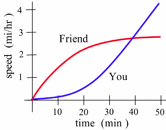
$A graph with the horizontal axis labeled "time (min)" and the vertical axis labeled "speed (mi/hr)." A blue curve labeled "You" starts at the origin a and initially rises slowly but steadily rises at a faster rate; a red curve labeled "Friend" starts at the origin and initially rises rpidly but steadily rises at a slower and slower rate. The curves cross at (40,3.5).$

Who is walking faster at $t = 20$?
Who is ahead at $t = 20$?
When are you and your friend farthest apart?
Who is ahead when $t = 50$?

Answer

Friend
Friend
At $t = 40$. Before that, your friend is walking faster and increasing the distance between you. Then you start to walk faster than your friend and start to catch up.
Friend. You are walking faster than your friend at $t = 50$, but you still have not caught up.

Example $\PageIndex{2}$

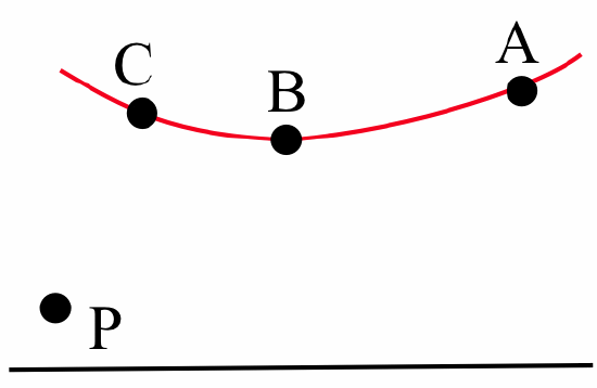
Which has the largest slope in the figure below: the line through the points $A$ and $P$, the line through $B$ and $P$, or the line through $C$ and $P$?

$A U-shaped curve starts above a point P, descends through C to a low point (still above P) at B, the begins rising and passes through A.$

Solution

The line through $C$ and $P$: $m_{PC} > m_{PB} > m_{PA}$.

Pratice $\PageIndex{4}$

In the figure below, the point $Q$ on the curve is fixed, and the point $P$ is moving to the right along the curve toward the point $Q$. As $P$ moves toward $Q$, is the indicated value increasing, decreasing, remaining constant, or doing something else?

$A curve in the first quadrant rises sharply through the point P, then continues to increase at a slower and slower rate before passing through Q and then beginning to flatten out.$

$x$-coordinate of $P$
$x$-increment from $P$ to $Q$
slope from $P$ to $Q$

Answer

The $x$-coordinate is increasing.
The $x$-increment $\Delta x$ is decreasing.
The slope of the line through $P$ and $Q$ is decreasing.

Example $\PageIndex{3}$

The graph of $y = f(x)$ appears below:

$A graph of y=f(x) starting near (-0.75,0) and curving upward through (1,0), reaching a peak at (2,2), falling steadily through (4,0) and reaching a low point (5,-1), then turning upward and passing through (6,-0.25). There is a line segment tangent to the graph at (1,0) that has slope 1, another at (2,2) that is horizontal, one at (3,1) with slope -1, and one that is horizontal at (5,-1).$

Let $g(x)$ be the slope of the line tangent to the graph of $f(x)$ at the point $(x,f(x))$.

Estimate the values $g(1)$, $g(2)$ and $g(3)$.
For what value(s) of $x$ is $g(x) = 0$?
At what value(s) of $x$ is $g(x)$ largest?
Sketch the graph of $y = g(x)$.

Solution

The figure shows the graph of $y = f(x)$ with several tangent lines to the graph of $f$. From this graph, we can estimate that $g(1)$ (the slope of the line tangent to the graph of $f$ at $(1,0)$) is approximately equal to $1$. Similarly, $g(2) \approx 0$ and $g(3) \approx -1$.
The slope of the tangent line appears to be horizontal (slope $= 0$) at $x = 2$ and at $x = 5$.
The tangent line to the graph of $f$ appears to have greatest slope (be steepest) near $x = 1.5$.

We can build a table of values of $g(x)$:

$x$	$f(x)$	$g(x)$
$0$	$-1.0$	$0.5$
$1$	$0.0$	$1.0$
$2$	$2.0$	$0.0$
$3$	$1.0$	$-1.0$
$4$	$0.0$	$-1.0$
$5$	$-1.0$	$0.0$
$6$	$-0.5$	$0.5$

and then sketch the graph of these values. A graph of $y = g(x)$ appears below:

$A graph labeled "g(x) = slope of f(x)" starting at (0,0.5), moving upward to (1,0.75), then moving sharply upward to a peak at (1.5,2), falling steadily through (2,0) and flattening from (2.5,-1) to (4,-1), then turning upward through (5,0) and flattening as it approaches (6,0.5).$

Practice $\PageIndex{5}$

Water flows into a container at a constant rate of $3$ gallons per minute into the container shown below:

$A container with symmetry about its central vertical axis. Water is flowing into the top and fills the container to a height h(t). The container is narrow at the bottom, flaring out to be very wide above that, then narrowing to a width slightly bigger than at the base, then flaring out a bit before narrowing again.$

Starting with an empty container, sketch the graph of the height of the water in the container as a function of time.

Answer: See the figure:
$An image showing a vase-like container being filled with water and the corresponding height versus time graph. The vase has sections labeled "fast," "slowest," and "slow" corresponding to the width of the container. The graph of water height over time shows that the slope (rate of height change) is slow when the vase is widest ("slowest" section), and fast when the vase is narrowest ("fast" sections), confirming the relationship between container width and filling speed.$

Problems

In Problems 1–4, match the numerical triples to the graphs. For example, in Problem 1, $A$: $3,~3,~6$ is “over and up” so it matches graph (a).

$A$: $3,~3,~6$; $B$: $12,~6,~6$; $C$: $7,~7,~3$ $D$: $2,~4,~4$
$Four piecewise-linear graphs (a, b, c, d) on a horizontal axis. Graph (a) is flat, then slopes up. Graph (b) slopes up, then is flat. Graph (c) slopes down, then is flat. Graph (d) is flat, then slopes down.$
$A$: $7,~10,~7$; $B$: $17,~17,~25$; $C$: $4,~4,~8$ $D$: $12,~8,~16$
$Four piecewise-linear graphs (a, b, c, d). Graph (a) is flat, then slopes up. Graph (b) is flat, then slopes up with a steeper slope. Graph (c) slopes down, then slopes up, forming a valley (V-shape). Graph (d) slopes up, then slopes down, forming a peak (inverted V-shape).$
$A$: $7,~14,~10$; $B$: $23,~45,~22$; $C$: $8,~12,~8$ $D$: $6,~9,~3$
$Four V-shaped graphs (a, b, c, d), all opening downward, resembling a reflected absolute value function. All graphs have a vertex near the top center, but (a) and (c) are slightly sharper, while (b) and (d) are slightly wider or flatter at the top.$
$A$: $6,~3,~9$; $B$: $8,~1,~1$; $C$: $12,~6,~9$ $D$: $3.7,~1.9,~3.6$
$Four V-shaped graphs (a, b, c, d), resembling a graph of absolute value function with shifts or reflections. Graph (a) opens up, with the vertex in the lower left. Graph (b) opens up, with the vertex centered low. Graph (c) opens up, with the vertex in the lower right. Graph (d) is flat, then slopes up.$
Water is flowing at a steady rate into each of the bottles shown below:
$Three containers (a, b, c): container (a) is cone-shaped (wide base, narrow top), container (b) is vase-shaped (narrow base, wide middle, narrow top), container (c) is hourglass-shaped (wide top, narrow middle, wide base). Below these are and three graphs showing height versus time when filling the containers: graph A (concave up, increasing slope), graph B (S-curve: concave up, then concave down) and Graph C (concave up, increasing slope).$
Match each bottle shape with the graph of the height of the water as a function of time
Sketch shapes of bottles that will have the water height versus time graphs shown below:
$Two graphs of height versus an independent variable (x or time). The graph on the left is an S-curve, showing a segment that is concave up, followed by a segment that is concave down, then concave up again. The graph on the right is a simple, increasing concave down curve, showing rapid initial growth that slows over time.$
If $f(x) = x^2 + 3$, $g(x) = \sqrt{x - 5}$ and $\displaystyle H(x) = \frac{x}{x - 2}$:
1. evaulate $f(1)$, $g(1)$ and $H(1)$.
2. graph $f(x)$, $g(x)$ and $H(x)$ for $-5 \leq x \leq 10$.
3. evaluate $f(3x)$, $g(3x)$ and $H(3x)$.
4. evaluate $f(x+h)$, $g(x+h)$ and $H(x+h)$.
Find the slope of the line through the points $P$ and $Q$ when:
1. $P = (1,3)$, $Q = (2,7)$
2. $P = (x, x^2 + 2)$, $Q = (x+h , (x+h)^2 + 2)$
3. $P = (1,3)$, $Q = (x, x^2 + 2)$
4. $P$, $Q$ as in (b) with $x=2$, $x=1.1$, $x=1.002$
Find the slope of the line through the points $P$ and $Q$ when:
1. $P = (1,5)$, $Q = (2,7)$
2. $P = (x, x^2 + 3x - 1)$, $Q = (x+h, (x+h)^2 + 3(x+h) - 1)$
3. $P$, $Q$ as in (b) with $x=1.3$, $x=1.1$, $x=1.002$
If $f(x) = x^2 + x$ and $g(x) = \frac{3}{x}$, evaluate and simplify $\displaystyle \frac{f(a+h) - f(a)}{h}$ and $\displaystyle \frac{g(a+h) - g(a)}{h}$ when $a = 1$, $a = 2$, $a = -1$, $a = x$.
If $f(x) = x^2 - 2x$ and $g(x) = \sqrt{x}$, evaluate and simplify $\displaystyle \frac{f(a+h) - f(a)}{h}$ and $\displaystyle \frac{g(a+h) - g(a)}{h}$ when $a = 1$, $a = 2$, $a = 3$, $a = x$.
The temperatures shown below were recorded during a 12-hour period in Chicago:
1. At what time was the temperature the highest? Lowest?
2. How fast was the temperature rising at 10 a.m.? At 1 p.m.?
3. What could have caused the drop in temperature between 1 p.m. and 3 p.m.?
The graph below shows the distance of an airplane from an airport during a long flight:
1. How far was the airplane from the airport at 1 p.m.? At 2 p.m.?
2. How fast was the distance changing at 1 p.m.?
3. How could the distance from the plane to the airport remain unchanged from 1:45 p.m. until 2:30 p.m. without the airplane falling?
The graph below shows the height of a diver above the water level at time $t$ seconds:
1. What was the height of the diving board?
2. When did the diver hit the water?
3. How deep did the diver get?
4. When did the diver return to the surface?
Refer to the curve shown below:
1. Sketch the lines tangent to the curve at $x = 1$, $2$, $3$, $4$ and $5$.
2. For what value(s) of $x$ is the value of the function largest? Smallest?
3. For what value(s) of $x$ is the slope of the tangent line largest? Smallest?
The figure below shows the height of the water (above and below mean sea level) at a Maine beach:
1. At which time(s) was the most beach exposed? The least?
2. At which time(s) was the current the strongest?
Imagine that you are ice skating, from left to right, along the path shown below:
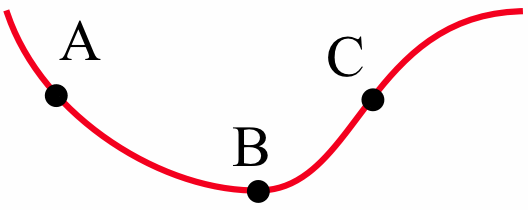
$A red concave-up curve that forms a valley, labeled with three points. Point A is on the left sloping down, Point B is at the bottom (minimum), and Point C is on the right sloping up.$
Sketch the path you will follow if you fall at points $A$, $B$ and $C$.
Define $s(x)$ to be the {\bf slope} of the line through the points $(0,0)$ and $(x, f(x))$ where $f(x)$ is the function graphed below:

For example, $s(3) =$ {\bf slope} of the line through $(0,0)$ and $(3, f(3))$ = $\frac43$.
1. Evaluate $s(1)$, $s(2)$ and $s(4)$.
2. For which integer value of $x$ between $1$ and $7$ is $s(x)$ smallest?
Let $f(x) = x + 1$ and define $s(x)$ to be the {\bf slope} of the line through the points $(0,0)$ and $(x, f(x))$, as shown below:

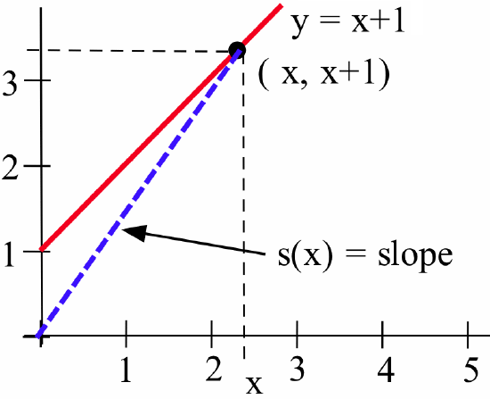
For example, $s(2) =$ slope of the line through $(0,0)$ and $(2,3)$ = $\frac32$.
1. Evaluate $s(1)$, $s(3)$ and $s(4)$.
2. Find a formula for $s(x)$.
Define $A(x)$ to be the area of the rectangle bounded by the coordinate axes, the line $y = 2$ and a vertical line at $x$, as shown below:

For example, $A(3) =$ area of a $2\times3$ rectangle $= 6$.
1. Evaluate $A(1)$, $A(2)$ and $A(5)$.
2. Find a formula for $A(x)$.

Using the graph of $y = f(x)$ below:
$A red curve y=f(x) plotted on a grid from x=0 to x=4. The curve passes through points (1,2), (2,2), (3,1), and (4,1.5).$
let $g(x)$ be the slope of the line tangent to the graph of $f(x)$ at the point $\left(x, f(x)\right)$. Complete the table, estimating values of the slopes as best you can.

$x$	$f(x)$	$g(x)$
$0$	$1$	$1$
$1$
$2$
$3$
$4$

Sketch the graphs of water height versus time for water pouring into a bottle shaped like:
1. a milk carton
2. a spherical glass vase
3. an oil drum (cylinder) lying on its side
4. a giraffe \item you
Design bottles whose graphs of (highest) water height versus time will look like those shown below:
$Two graphs of height versus time. The graph on the left is a single straight line rising from the origin. The graph on the right is a piecewise linear graph; it rises linearly, then is flat (constant height), and then rises linearly again with a steeper slope.$

Input (\(x\))	Output (\(x^2\))
\(x\)	\(x^2\)
\(a\)	\(a^2\)
\(2.5\)	\(6.25\)
\(x+h\)	\((x+h)^2\)

input	output
\(x\)	\(\frac{3}{x}+1\)
\(5\)	\(\frac35 + 1 = 1.6\)
\(a\)	\(\frac{3}{a}+1\)
\(c+3\)	\(\frac{3}{c+3}+1\)
\(x+h\)	\(\frac{3}{x+h}+1\)

\(x\)	\(f(x)\)	\(g(x)\)
\(0\)	\(-1.0\)	\(0.5\)
\(1\)	\(0.0\)	\(1.0\)
\(2\)	\(2.0\)	\(0.0\)
\(3\)	\(1.0\)	\(-1.0\)
\(4\)	\(0.0\)	\(-1.0\)
\(5\)	\(-1.0\)	\(0.0\)
\(6\)	\(-0.5\)	\(0.5\)

\(x\)	\(f(x)\)	\(g(x)\)
\(0\)	\(1\)	\(1\)
\(1\)
\(2\)
\(3\)
\(4\)

Search

Text Color

Text Size

Margin Size

Font Type

Definition

Practice \(\PageIndex{1}\)

Practice \(\PageIndex{2}\)

Vertical Line Test for a Function

Example \(\PageIndex{1}\)

Solution

Practice \(\PageIndex{3}\)

Example \(\PageIndex{2}\)

Solution

Pratice \(\PageIndex{4}\)

Example \(\PageIndex{3}\)

Solution

Practice \(\PageIndex{5}\)