1.2: Properties of Limits

This section presents results that make it easier to calculate limits of combinations of functions or to show that a limit does not exist. The main result says we can determine the limit of “elementary combinations” of functions by calculating the limit of each function separately and recombining these results to get our final answer.

Main Limit Theorem

If \(\displaystyle \lim_{x \to a} \, f(x) = L\) and \(\displaystyle \lim_{x\to a} \, g(x) = M\) then:

1. \(\displaystyle \lim_{x \to a} \, \left[f(x) + g(x)\right] = L+M\)
2. \(\displaystyle \lim_{x \to a} \, \left[f(x) - g(x)\right] = L-M\)
3. \(\displaystyle \lim_{x \to a} \, k \cdot f(x) = k \cdot L\)
4. \(\displaystyle \lim_{x \to a} \, f(x) \cdot g(x) = L\cdot M\)
5. \(\displaystyle \lim_{x \to a} \, \frac{f(x)}{g(x)} = \frac{L}{M} \quad \left(\mbox{if }M\neq 0\right)\)
6. \(\displaystyle \lim_{x \to a} \, \left[f(x)\right]^n = L^n\)
7. \(\displaystyle \lim_{x \to a} \, \sqrt[n]{f(x)} = \sqrt[n]{L}\)

When \(n\) is an even integer in part (g), we need \(L\geq 0\) and \(f(x) \geq 0\) for \(x\) near \(a\).

The Main Limit Theorem says we get the same result if we first perform the algebra and then take the limit or if we take the limits first and then perform the algebra: for example, (a) says that the limit of the sum equals the sum of the limits.

A proof of the Main Limit Theorem is not inherently difficult, but it requires a more precise definition of the limit concept than we have at the moment, and it then involves a number of technical difficulties. 

Practice \(\PageIndex{1}\)

For\(f(x) = x^2 - x - 6\) and\(g(x) = x^2 - 2x - 3\), evaluate:

1. \(\displaystyle \lim_{x\to 1} \, \left[f(x) + g(x)\right]\)
2. \(\displaystyle \lim_{x\to 1} \, f(x) \cdot g(x)\)
3. \(\displaystyle \lim_{x\to 1} \, \frac{f(x)}{g(x)}\)
4. \(\displaystyle \lim_{x\to 3} \, \left[f(x) + g(x)\right]\)
5. \(\displaystyle \lim_{x\to 3} \, f(x) \cdot g(x)\)
6. \(\displaystyle \lim_{x\to 3} \, \frac{f(x)}{g(x)}\)
7. \(\displaystyle \lim_{x\to 2} \, \left[f(x)\right]^3\)
8. \(\displaystyle \lim_{x\to 2} \, \sqrt{1-g(x)}\)

Answer

1. \(-10\)
2. \(24\)
3. \(\frac32\)
4. \(0\)
5. \(0\)
6. \(\frac54\)
7. \(-64\)
8. \(2\)

Limits of Some Very Nice Functions: Substitution

As you may have noticed in the previous example, for some functions \(f(x)\) it is possible to calculate the limit as\(x\) approaches\(a\) simply by substituting\(x = a\) into the function and then evaluating\(f(a)\), but sometimes this method does not work. The following results help to (partially) answer the question about when such a substitution is valid.

Two Easy Limits

\(\displaystyle \lim_{x\to a} \, k = k\) and \(\displaystyle \lim_{x\to a} \, x = a\)

We can use the preceding Two Easy Limits and the Main Limit Theorem to prove the following Substitution Theorem.

Substitution Theorem For Polynomial and Rational Functions

If: \(P(x)\) and \(Q(x)\) are polynomials and \(a\) is any number

then: \(\displaystyle \lim_{x\to a} \, P(x) = P(a)\) and \(\displaystyle \lim_{x\to a} \, \frac{P(x)}{Q(x)} = \frac{P(a)}{Q(a)}\) (as long as\(Q(a) \neq 0\)).

The Substitution Theorem says that we can calculate the limits of polynomials and rational functions by substituting (as long as the substitution does not result in a division by \(0\)).

Practice \(\PageIndex{2}\)

Evaluate each limit.

1. \(\displaystyle \lim_{x\to 2} \, \left[5x^3 - x^2 + 3\right]\)
2. \(\displaystyle \lim_{x\to 2} \, \frac{x^3 - 7x}{x^2 + 3x}\)
3. \(\displaystyle \lim_{x\to 2} \, \frac{x^2 - 2x}{x^2 -x-2}\)

Answer

1. \(39\)
2. \(-\frac35\)
3. \(\frac23\)

Limits of Other Combinations of Functions

So far we have concentrated on limits of single functions and elementary combinations of functions. If we are working with limits of other combinations or compositions of functions, the situation becomes slightly more difficult, but sometimes these more complicated limits have useful geometric interpretations.

Example \(\PageIndex{1}\)

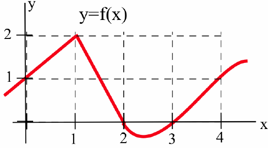
Use the graph below to estimate each limit.

1. \(\displaystyle \lim_{x\to 1} \, \left[3+f(x)\right]\)
2. \(\displaystyle \lim_{x\to 1} \, f(2+x)\)
3. \(\displaystyle \lim_{x\to 0} \, f(3-x)\)
4. \(\displaystyle \lim_{x\to 2} \, \left[f(x+1)-f(x)\right]\)

Solution

1. \(\displaystyle \lim_{x\to 1} \, \left[3+f(x)\right]\) requires a straightforward application of part (a) of the Main Limit Theorem:\[\lim_{x\to 1} \, \left[3+f(x)\right] = \lim_{x\to 1} \, 3 + \lim_{x\to 1} \, f(x) = 3 + 2 = 5\nonumber\]
2. We first need to examine what happens to the quantity\(2+x\) as\(x\rightarrow 1\) before we can consider the limit of\(f(2+x)\). When\(x\) is very close to \(1\), the value of \(2+x\) is very close to \(3\), so the limit of \(f(2+x)\) as\(x\rightarrow 1\) is equivalent to the limit of \(f(w)\) as \(w\rightarrow 3\) (where \(w=2+x\)) and it is clear from the graph that \(\displaystyle \, \lim_{w\to 3} f(w) = 1\), so:\[\lim_{x\to 1} \, f(2+x) = \displaystyle \lim_{w\to 3} \, f(w) = 1\nonumber\]In most situations it is not necessary to formally substitute a new variable \(w\) for the quantity \(2+x\), but it is still necessary to think about what happens to the quantity \(2+x\) as \(x\rightarrow 1\).
3. As \(x\rightarrow 0\) the quantity \(3-x\) will approach \(3\), so we want to know what happens to the values of \(f\) when the input variable is approaching \(3\):\[\lim_{x\to 0} \, f(3-x) = 1\nonumber\]
4. Using part (b) of the Main Limit Theorem: \begin{align*} \lim_{x\to 2} \, \left[f(x+1)-f(x)\right] &= \lim_{x\to 2} \, f(x+1) - \lim_{x\to 2} \, f(x)\\ &= \lim_{w\to 3} \, f(w) - \lim_{x\to 2} \, f(x) = 1 - 3 = -2 \end{align*} (Notice the use of the substitution \(w =x+1\) above.)

Practice \(\PageIndex{3}\)

Use the graph below to estimate each limit.

1. \(\displaystyle \lim_{x\to 1} \, f(2x)\)
2. \(\displaystyle \lim_{x\to 2} \, f(x-1)\)
3. \(\displaystyle \lim_{x\to 0} \, 3\cdot f(4+x)\)
4. \(\displaystyle \lim_{x\to 2} \, f(3x-2)\)

Answer

1. \(0\)
2. \(2\)
3. \(3\)
4. \(1\)

Example \(\PageIndex{2}\)

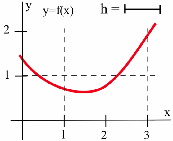
Use the graph below to estimate each limit.

1. \(\displaystyle \lim_{h\to 0} \, f(3+h)\)
2. \(\displaystyle \lim_{h\to 0} \, f(3)\)
3. \(\displaystyle \lim_{h\to 0} \, \left[f(3+h)-f(3)\right]\)
4. \(\displaystyle \lim_{h\to 0} \, \frac{f(3+h)-f(3)}{h}\)

The last limit is a special type of limit we will encounter often in this book, while the first three parts are the steps we need to evaluate it.

Solution

1. As \(h\rightarrow 0\), the quantity \(w = 3+h\) will approach \(3\), so\[\lim_{h\to 0} \, f(3+h) = \lim_{w\to 3}\, f(w) = 1\nonumber\]
2. \(f(3)\) is a constant (equal to \(1\)) and does not depend on \(h\) in any way, so:\[\lim_{h\to 0} \, f(3) = f(3) = 1\nonumber\]
3. This limit is just an algebraic combination of the first two limits:\[\lim_{h\to 0} \, \left[f(3+h)-f(3)\right] = \lim_{h\to 0} \, f(3+h) - \lim_{h\to 0}\, f(3) = 1-1 = 0\nonumber\]The quantity \(f(3+h) - f(3)\) also has a geometric interpretation: it is the change in the \(y\)-coordinates, the \(\Delta y\), between the points \((3,f(3))\) and \((3+h,f(3+h))\):
   
4. As \(h\rightarrow 0\), the numerator and denominator of \(\displaystyle \frac{f(3+h) - f(3)}{h}\) both approach \(0\), so we cannot immediately determine the value of the limit. But if we recognize that \(f(3+h) - f(3) = \Delta y\) for the two points \((3, f(3))\) and \((3+h, f(3+h))\) and that \(h = \Delta x\) for the same two points, then we can interpret \(\displaystyle \frac{f(3+h) - f(3)}{h}\) as \(\frac{\Delta y}{\Delta x}\), which is the slope of the secant line through the two points: \begin{align*} \lim_{h \to 0} \, \frac{f(3+h) - f(3)}{h} &= \lim_{\Delta x \to 0} \, \left[\mbox{slope of the secant line}\right] \\ &= \mbox{slope of the tangent line at }(3, f(3))\\ &\approx -1 \end{align*} This last limit represents the slope of line tangent to the graph of \(f\) at the point \(( 3, f(3) )\). (It is a pattern we will encounter often.)

Tangent Lines as Limits

If we have two points on the graph of the function \(y = f(x)\):\[(x, f(x)) \mbox{ and } ( x+h, f(x+h) )\nonumber\]then \(\Delta y = f(x+h) - f(x)\) and\(\Delta x = (x+h) - (x) = h\), so the slope of the secant line through those points is:\[m_{\mbox{sec}} = \frac{\Delta y}{\Delta x}\nonumber\]and the slope of the line tangent to the graph of \(f\) at the point \(( x, f(x) )\) is, by definition,\[m_{\mbox{tan}} = \lim_{\Delta x \to 0} \, \left[\mbox{slope of the secant line}\right] = \lim_{h \to 0} \, \frac{f(x + h) - f(x)}{h}\nonumber\]
 

Example \(\PageIndex{3}\)

Give a geometric interpretation for the following limits and estimate their values for the function whose graph appears below.

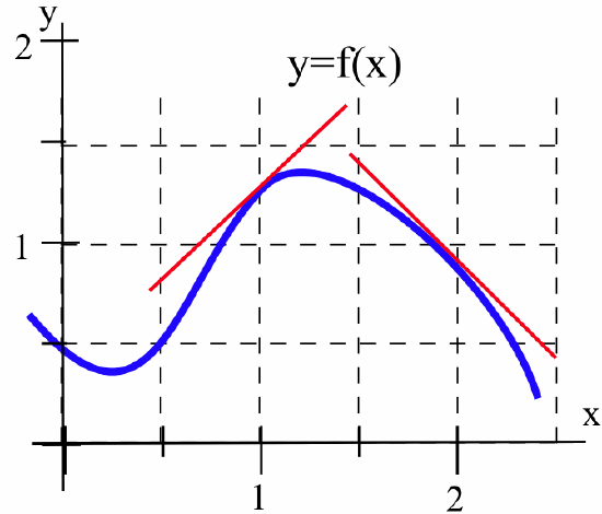
1. \(\displaystyle \lim_{h\to 0} \, \frac{f(1+h)-f(1)}{h}\)
2. \(\displaystyle \lim_{h\to 0} \, \frac{f(2+h)-f(2)}{h}\)

Solution

1. The limit represents the slope of the line tangent to the graph of \(f(x)\) at the point \((1, f(1))\), so \(\displaystyle \lim_{h\to 0} \, \frac{f(1+h)-f(1)}{h} \approx 1\).
2. The limit represents the slope of the line tangent to the graph of \(f(x)\) at the point \((2, f(2))\), so \(\displaystyle \lim_{h\to 0} \, \frac{f(2+h)-f(2)}{h} \approx -1\).

Practice \(\PageIndex{4}\)

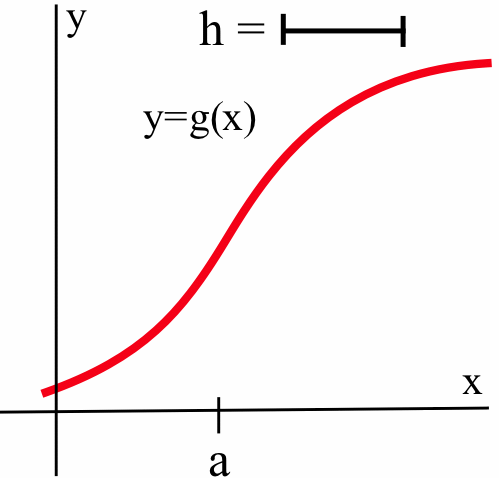
Give a geometric interpretation for the following limits and estimate their values for the function whose graph appears below.

1. \(\displaystyle \lim_{h\to 0} \, \frac{g(1+h)-g(1)}{h}\)
2. \(\displaystyle \lim_{h\to 0} \, \frac{g(3+h)-g(3)}{h}\)
3. \(\displaystyle \lim_{h\to 0} \, \frac{g(h)-g(0)}{h}\)

Answer

1. slope of the line tangent to the graph of \(g\) at the point \((1,g(1))\); estimated slope \(\approx -2\)
2. slope of the line tangent to the graph of \(g\) at the point \((3,g(3))\); estimated slope \(\approx 0\)
3. slope of the line tangent to the graph of \(g\) at the point \((0, g(0))\); estimated slope \(\approx 1\)

Comparing the Limits of Functions

Sometimes it is difficult to work directly with a function. However, if we can compare our complicated function with simpler ones, then we can use information about the simpler functions to draw conclusions about the complicated one. If the complicated function is always between two functions whose limits are equal, then we know the limit of the complicated function.

Squeezing Theorem

If: \(g(x) \leq f(x) \leq h(x)\) for all \(x\) near (but not equal to) \(c\)

and: \(\displaystyle \lim_{x\to c} \, g(x) = \lim_{x\to c} \, h(x) = L\)

then: \(\displaystyle \lim_{x\to c} \, f(x) = L\).

The figure below shows the idea behind the proof of this theorem:

The function \(f(x)\) gets “squeezed” between the smaller function \(g(x)\) and the bigger function \(h(x)\). Because \(g(x)\) and \(h(x)\) converge to the same limit, \(L\), so must \(f(x)\).

We can use the Squeezing Theorem to evaluate some “hard” limits by squeezing a “complicated” function in between two “simpler” functions with “easier” limits.

Example \(\PageIndex{4}\)

Use the inequality \(-\left|x\right| \leq \sin(x) \leq \left|x\right|\) to determine:

1. \(\displaystyle \lim_{x\to 0} \, \sin(x)\)
2. \(\displaystyle \lim_{x\to 0} \, \cos(x)\)

Solution

1. \(\displaystyle \lim_{x\to 0} \, \left|x\right| = 0\) and \(\displaystyle \lim_{x\to 0} \, -\left|x\right| = 0\) so, by the Squeezing Theorem, \(\displaystyle \lim_{x\to 0} \, \sin(x) = 0\).
2. If \(-\frac{\pi}{2} < x < \frac{\pi}{2}\), then \(\cos(x) = \sqrt{1 - \sin^2(x)}\), so \(\displaystyle \lim_{x\to 0} \, \cos(x) = \lim_{x\to 0} \, \sqrt{1 - \sin^2(x)} = \sqrt{1-0^2} = 1\).

Example \(\PageIndex{5}\)

Evaluate \(\displaystyle \lim_{x\to 0} \, x\cdot \sin\left(\frac{1}{x}\right)\).

Solution

In the graph of \(\sin\left(\frac{1}{x}\right)\):

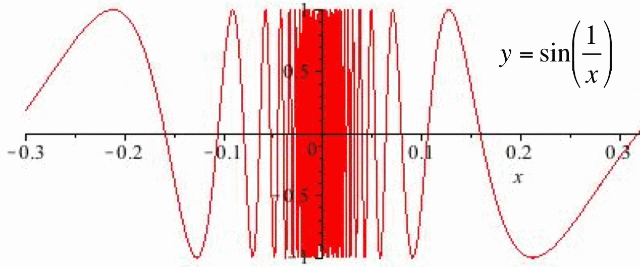
the \(y\)-values change very rapidly for values of \(x\) near \(0\), but they all lie between \(-1\) and \(1\):\[-1 \leq \sin\left(\frac{1}{x}\right) \leq 1\nonumber\]so, if \(x > 0\), multiplying this inequality by \(x\) we get:\[-x \leq x \cdot \sin\left(\frac{1}{x}\right) \leq x\nonumber\]which we can rewrite as:\[-\left|x\right| \leq x \cdot \sin\left(\frac{1}{x}\right) \leq \left|x\right|\nonumber\]because \(\left|x\right| = x\) when \(x > 0\).

If \(x < 0\), when we multiply the original inequality by \(x\) we get:\[-x \geq x \cdot \sin\left(\frac{1}{x}\right) \geq x \quad \Rightarrow \quad \left|x\right| \geq x \cdot \sin\left(\frac{1}{x}\right) \geq -\left|x\right|\nonumber\]because \(\left|x\right| = -x\) when \(x<0\). Either way we have:\[-\left|x\right| \leq x \cdot \sin\left(\frac{1}{x}\right) \leq \left|x\right|\nonumber\] for all \(x \neq 0\), and in particular for \(x\) near \(0\).

Both “simple” functions (\(-\left|x\right|\) and \(\left|x\right|\)) approach \(0\) as \(x\rightarrow 0\), so \[\lim_{x \to 0} \, x \cdot \sin\left(\frac{1}{x}\right) = 0\nonumber\]by the Squeezing Theorem.

Practice \(\PageIndex{5}\)

If \(f(x)\) is always between \(x^2 + 2\) and \(2x + 1\), what can you say about \(\displaystyle \lim_{x\to 1} \, f(x)\)?

Answer

\(\displaystyle \lim_{x\to 1} \, \left[x^2 + 2\right] = 3\) and \(\displaystyle \lim_{x\to 1} \, \left[2x+1\right] = 3\) so \(\displaystyle \lim_{x\to 1} \, f(x) = 3\)

Practice \(\PageIndex{6}\)

Use the relation \(\cos(x) \leq \frac{\sin(x)}{x} \leq 1\) (Problem 27 guides you through the steps to prove this relation) to show that:\[\lim_{x\to 0} \, \frac{\sin(x)}{x} = 1\nonumber\]

Answer

\(\displaystyle \lim_{x\to 0} \, \cos(x) = 1\) and \(\displaystyle \lim_{x\to 0} \, 1 = 1\) so \(\displaystyle \lim_{x\to 0} \, \frac{\sin(x)}{x} = 1\)

List Method for Showing that a Limit Does Not Exist

If the limit of \(f(x)\), as \(x\) approaches \(c\), exists and equals \(L\), then we can guarantee that the values of \(f(x)\) are as close to \(L\) as we want by restricting the values of \(x\) to be very, very close to \(c\). To show that a limit, as \(x\) approaches \(c\), does not exist, we need to show that no matter how closely we restrict the values of \(x\) to \(c\), the values of \(f(x)\) are not all close to a single, finite value \(L\).

One way to demonstrate that \(\displaystyle \lim_{x\to c} \, f(x)\) does not exist is to show that the left and right limits exist but are not equal.

Another method of showing that \(\displaystyle \lim_{x\to c} \, f(x)\) does not exist uses two (infinite) lists of numbers, \(\left\{a_1, a_2, a_3, a_4,\ldots\right\}\) and \(\left\{b_1, b_2, b_3, b_4,\ldots\right\}\), with entries that become arbitrarily close to the value \(c\) as the subscripts get larger, but for which the corresponding lists of function values, \(\left\{f(a_1), f(a_2), f(a_3), f(a_4),\ldots\right\}\) and \(\left\{f(b_1), f(b_2), f(b_3), f(b_4),\ldots\right\}\) approach two different numbers as the subscripts get larger.

Example \(\PageIndex{6}\)

For \(f(x)\) defined as:\[f(x) = \left\{
\begin{array}{rl}
{1} & {\text{if } x < 1 } \\
{x} & {\text{if } 1 < x < 3 }\\
{2} & {\text{if } 3 < x }\end{array}\right.\nonumber\]show that \(\displaystyle \lim_{x\to 3} \, f(x)\) does not exist.

Solution

We could use one-sided limits to show that this limit does not exist, but instead we will use the list method.

One way to define values of \(\left\{a_1, a_2, a_3, a_4,\ldots\right\}\) that approach \(3\) from the right is to define \(a_1 = 3 + 1\), \(a_2 = 3 + \frac12\), \(a_3 = 3 + \frac13\), \(a_4 = 3 + \frac14\) and, in general, \(a_n = 3 + \frac{1}{n}\). Then \(a_n > 3\) so \(f(a_n) = 2\) for all subscripts \(n\), and the values in the list \(\left\{f(a_1), f(a_2), f(a_3), f(a_4),\ldots\right\}\) are all close to \(2\) — in fact, all of the \(f(a_n)\) values equal \(2\).

We can define values of \(\left\{b_1, b_2, b_3, b_4,\ldots\right\}\) that approach \(3\) from the left by \(b_1 = 3 - 1\), \(b_2 = 3 - \frac12\), \(b_3 = 3 - \frac13\), \(b_4 = 3 - \frac14\), and, in general, \(b_n = 3 - \frac{1}{n}\). Then \(b_n < 3\) so \(f(b_n) = b_n = 3 - \frac{1}{n}\) for each subscript \(n\), and the values in the list \(\left\{f(b_1), f(b_2), f(b_3), f(b_4),\ldots\right\} = \left\{2, 2.5, 2\frac23, 2\frac34, 2\frac45,\ldots , 3 - \frac{1}{n},\ldots\right\}\) are all close to \(3\) for large values of \(n\).

Because the values in the lists \(\left\{f(a_1), f(a_2), f(a_3), f(a_4),\ldots\right\}\) and  \(\left\{f(b_1), f(b_2), f(b_3), f(b_4),\ldots\right\}\) have two different limiting values, we can conclude that \(\displaystyle \lim_{x\to 3} \, f(x)\) does not exist.

Example \(\PageIndex{7}\)

Define \(h(x)\) as:\[h(x) = \left\{
\begin{array}{rl}
{2} & {\text{if }x\text{ is a rational number}}\\
{1} & {\text{if }x\text{ is an irrational number}}\end{array}\right.\nonumber\](the “holey” function introduced in Section 0.4). Use the list method to show that \(\displaystyle \lim_{x\to 3} \, h(x)\) does not exist.

Solution

Let \(\left\{a_1, a_2, a_3, a_4,\ldots\right\}\) be a list of rational numbers that approach \(3\): for example, \(a_1 = 3 + 1\), \(a_2 = 3 + \frac12\), \(a_3 = 3 + \frac13\), … , \(a_n = 3 + \frac{1}{n}\). Then \(f(a_n) =2\) for all \(n\), so:\[\left\{f(a_1), f(a_2), f(a_3), f(a_4),\ldots\right\} = \left\{2, 2, 2, 2,\ldots\right\}\nonumber\]and the \(f(a_n)\) values are all “close to” (in fact, equal) \(2\).

If \(\left\{b_1, b_2, b_3, b_4,\ldots\right\}\) is a list of irrational numbers that approach \(3\) (for example, \(b_1 = 3 + \pi\), \(b_2 = 3 + \frac{\pi}{2}\), …, \(b_n = 3 + \frac{\pi}{n}\)) then:\[\left\{f(b_1), f(b_2), f(b_3), f(b_4),\ldots\right\} = \left\{1, 1, 1, 1,\ldots\right\}\nonumber\]and the \(f(b_n)\) values are all close to \(1\) for large values of \(n\).

Because the \(f(a_n)\) and \(f(b_n)\) values become close to two different numbers, the limit of \(f(x)\) as \(x\rightarrow 3\) does not exist. A similar argument will work as \(x\) approaches any number \(c\), so for every \(c\) we can show that \(\displaystyle \lim_{x\to c} \, (x)\) does not exist. The “holey” function does not have a limit as \(x\) approaches any value \(c\).

Problems

1. Use the functions \(f\) and \(g\) defined by the graphs below to determine the following limits.
   
   1. \(\displaystyle \lim_{x \to 1} \, \left[f(x) + g(x)\right]\)
   2. \(\displaystyle \lim_{x \to 1} \, f(x) \cdot g(x)\)
   3. \(\displaystyle \lim_{x \to 1} \, \frac{f(x)}{g(x)}\)
   4. \(\displaystyle \lim_{x \to 1} \, f(g(x))\)
2. Use the functions \(f\) and \(g\) defined by the graphs in Problem 1 to determine the following limits.
   1. \(\displaystyle \lim_{x \to 2} \, \left[f(x) + g(x)\right]\)
   2. \(\displaystyle \lim_{x \to 2} \, f(x) \cdot g(x)\)
   3. \(\displaystyle \lim_{x \to 2} \, \frac{f(x)}{g(x)}\)
   4. \(\displaystyle \lim_{x \to 2} \, f(g(x))\)
3. Use the function \(h\) defined by the graph below to determine the following limits.
   
   1. \(\displaystyle \lim_{x \to 2} \, h(2x-2)\)
   2. \(\displaystyle \lim_{x \to 2} \, \left[x+h(x)\right]\)
   3. \(\displaystyle \lim_{x \to 2} \, h(1+x)\)
   4. \(\displaystyle \lim_{x \to 3} \, h\left(\frac{x}{2}\right)\)
4. Use the function \(h\) defined by the graph in Problem 3 to determine the following limits.
   1. \(\displaystyle \lim_{x \to 2} \, h(5-x)\)
   2. \(\displaystyle \lim_{x \to 0} \, \left[h(3+x)-h(3)\right]\)
   3. \(\displaystyle \lim_{x \to 2} \, x\cdot h(x-1)\)
   4. \(\displaystyle \lim_{x \to 0} \, \frac{h(3+x)-h(3)}{x}\)
5. Label the parts of the graph of \(f\) (below):
   
   that are described by:
   1. \(\displaystyle 2 + h\)
   2. \(\displaystyle f(2 )\)
   3. \(\displaystyle f(2 + h)\)
   4. \(\displaystyle f(2 + h) - f(2)\)
   5. \(\displaystyle \frac{f(2 + h) - f(2)}{(2+h)-2}\)
   6. \(\displaystyle \frac{f(2 - h) - f(2)}{(2-h)-2}\)
6. Label the parts of the graph of \(g\) (below):
   
   that are described by:
   1. \(\displaystyle a + h\)
   2. \(\displaystyle g(a)\)
   3. \(\displaystyle g(a + h)\)
   4. \(\displaystyle g(a + h) - g(a)\)
   5. \(\displaystyle \frac{g(a + h) - g(a)}{(a+h)-a}\)
   6. \(\displaystyle \frac{g(a - h) - g(a)}{(a-h)-a}\)
7. Use the graph below to estimate each limit:
   
   1. \(\displaystyle \lim_{x\to 1^{+}} \, f(x)\)
   2. \(\displaystyle \lim_{x\to 1^{-}} \, f(x)\)
   3. \(\displaystyle \lim_{x\to 1} \, f(x)\)
   4. \(\displaystyle \lim_{x\to 3^{+}} \, f(x)\)
   5. \(\displaystyle \lim_{x\to 3^{-}} \, f(x)\)
   6. \(\displaystyle \lim_{x\to 3} \, f(x)\)
   7. \(\displaystyle \lim_{x\to -1^{+}} \, f(x)\)
   8. \(\displaystyle \lim_{x\to -1^{-}} \, f(x)\)
   9. \(\displaystyle \lim_{x\to -1} \, f(x)\)
8. Use the graph from Problem 7 to estimate:
   1. \(\displaystyle \lim_{x\to 2^{+}} \, f(x)\)
   2. \(\displaystyle \lim_{x\to 2^{-}} \, f(x)\)
   3. \(\displaystyle \lim_{x\to 2} \, f(x)\)
   4. \(\displaystyle \lim_{x\to 4^{+}} \, f(x)\)
   5. \(\displaystyle \lim_{x\to 4^{-}} \, f(x)\)
   6. \(\displaystyle \lim_{x\to 4} \, f(x)\)
   7. \(\displaystyle \lim_{x\to -2^{+}} \, f(x)\)
   8. \(\displaystyle \lim_{x\to -2^{-}} \, f(x)\)
   9. \(\displaystyle \lim_{x\to -2} \, f(x)\)
9. The Lorentz contraction formula in relativity theory says the length \(L\) of an object moving at \(v\) miles per second with respect to an observer is:\[ L = A\cdot \sqrt{1 - \frac{v^2}{c^2}}\nonumber\]where \(c\) is the speed of light (a constant).
   1. Determine the object’s “rest length” (\(v = 0\)).
   2. Determine: \(\displaystyle \lim_{v\to c^{-}} \, L\)
10. Evaluate each limit.
    1. \(\displaystyle \lim_{x\to 2^{+}} \, \left\lfloor x\right\rfloor\)
    2. \(\displaystyle \lim_{x\to 2^{-}} \, \left\lfloor x\right\rfloor\)
    3. \(\displaystyle \lim_{x\to -2^{+}} \, \left\lfloor x\right\rfloor\)
    4. \(\displaystyle \lim_{x\to -2^{-}} \, \left\lfloor x\right\rfloor\)
    5. \(\displaystyle \lim_{x\to -2.3} \, \left\lfloor x \right\rfloor\)
    6. \(\displaystyle \lim_{x\to 3} \, \left\lfloor \frac{x}{2}\right\rfloor\)
    7. \(\displaystyle \lim_{x\to 3} \, \frac{\left\lfloor x\right\rfloor}{2}\)
    8. \(\displaystyle \lim_{x\to 0^{+}} \, \frac{\left\lfloor 2+x\right\rfloor - \left\lfloor 2\right\rfloor}{x}\)
11. For \(f(x)\) and \(g(x)\) defined as:\[
12. For \(f(x)\) and \(g(x)\) defined as:\[ f(x) = \left\{ \begin{array}{rl} { 1 } & { \text{if } x < 1} \\ { x } & { \text{if } 1 < x }\end{array}\right. \qquad g(x) = \left\{ \begin{array}{rl} { x } & { \text{if } x \neq 2 }\\ { 3 } & { \text{if } x = 2 }\end{array}\right.\nonumber\] determine the following limits:
    1. \(\displaystyle \lim_{x\to 2} \, \left[f(x)+g(x)\right]\)
    2. \(\displaystyle \lim_{x\to 2} \, \frac{f(x)}{g(x)}\)
    3. \(\displaystyle \lim_{x\to 2} \, f(g(x))\)
    4. \(\displaystyle \lim_{x\to 0} \, \frac{g(x)}{f(x)}\)
    5. \(\displaystyle \lim_{x\to 1} \, \frac{f(x)}{g(x)}\)
    6. \(\displaystyle \lim_{x\to 1} \, g(f(x))\)
13. Give geometric interpretations for each limit and use a calculator to estimate its value.
    
    1. \(\displaystyle \lim_{h\to 0} \, \frac{\arctan(0+ h) - \arctan(0)}{h}\)
    2. \(\displaystyle \lim_{h\to 0} \, \frac{\arctan(1+ h) - \arctan(1)}{h}\)
    3. \(\displaystyle \lim_{h\to 0} \, \frac{\arctan(2+ h) - \arctan(2)}{h}\)
14. 1. What does \(\displaystyle \lim_{h\to 0} \, \frac{\cos(h)-1}{h}\) represent in relation to the graph of \(y = \cos(x)\)? It may help to recognize that:\[\frac{\cos(h) - 1}{h} = \frac{\cos(0 + h) - \cos(0)}{h}\nonumber\]
    2. Graphically and using your calculator, estimate \(\displaystyle \lim_{h\to 0} \, \frac{\cos(h)-1}{h}\).
15. 1. What does the ratio \(\displaystyle \frac{\ln(1 + h)}{h}\) represent in relation to the graph of \(y = \ln(x)\)? It may help to recognize that:\[\frac{\ln(1+h)}{h} = \frac{\ln(1 + h) - \ln(1)}{h}\nonumber\]
    2. Graphically and using your calculator, determine \(\displaystyle \lim_{h\to 0} \, \frac{\ln(1 + h)}{h}\).
16. Use your calculator (to generate a table of values) to help you estimate the value of each limit.
    1. \(\displaystyle \lim_{h\to 0} \, \frac{e^h - 1}{h}\)
    2. \(\displaystyle \lim_{c\to 0} \, \frac{\tan(1+c) - \tan(1)}{c}\)
    3. \(\displaystyle \lim_{t\to 0} \, \frac{g(2+t) - g(2)}{t}\) when \(g(t) = t^2 - 5\).
17. 1. For \(h > 0\), find the slope of the line through the points \(( h, \left| h \right| )\) and \(( 0,0 )\).
    2. For \(h < 0\), find the slope of the line through the points \(( h, \left| h \right| )\) and \(( 0,0 )\).
    3. Evaluate \(\displaystyle \lim_{h\to 0^{-}} \, \frac{\left|h \right|}{h}\), \(\displaystyle \lim_{h\to 0^{+}} \, \frac{\left|h \right|}{h}\) and \(\displaystyle \lim_{h\to 0} \, \frac{\left|h \right|}{h}\).

In 17–18, describe the behavior at each integer of the function \(y = f(x)\) in the figure provided, using one of these phrases:

• “connected and smooth”
• “connected with a corner”
• “not connected because of a simple hole that could be plugged by adding or moving one point”
• “not connected because of a vertical jump that could not be plugged by moving one point”

17. 
18. 
19. Use the list method to show that \(\displaystyle \lim_{x\to 2} \, \frac{\left| x -2 \right|}{x - 2}\) does not exist.
20. Show that \(\displaystyle \lim_{x\to 0} \, \sin\left(\frac{1}{x}\right)\) does not exist. (Suggestion: Let \(f(x) = \sin\left(\frac{1}{x}\right)\) and let \(a_n = \frac{1}{n\pi}\) so that \(f(a_n) = \sin\left(\frac{1}{a_n}\right) = \sin(n\pi) = 0\) for every \(n\). Then pick \(b_n = \frac{1}{2n\pi + \frac{\pi}{2}}\) so that \(f(b_n) = \sin\left(\frac{1}{b_n}\right) = \sin(2n\pi + \frac{\pi}{2}) = \sin(\frac{\pi}{2}) = 1\) for all \(n\).)

In Problems 21–26, use the Squeezing Theorem to help evaluate each limit.

26. \(\displaystyle \lim_{x \to 0} \, x^2\cos\left(\frac{1}{x^2}\right)\)
27. \(\displaystyle \lim_{x \to 0} \, \sqrt[3]{x}\sin\left(\frac{1}{x^3}\right)\)
28. \(\displaystyle \lim_{x \to 0}\, 3+x^2\sin\left(\frac{1}{x}\right)\)
29. \(\displaystyle \lim_{x \to 1^{-}} \sqrt{1-x^2}\cos\left(\frac{1}{x-1}\right)\)
30. \(\displaystyle \lim_{x \to 0} \, x^2\cdot \left\lfloor \frac{1}{x^2} \right\rfloor\)
31. \(\displaystyle \lim_{x \to 0} \, (-1)^{\left\lfloor \frac{1}{x} \right\rfloor}\left(1-\cos(x)\right)\)
32. This problem outlines the steps of a proof that \(\displaystyle \lim_{\theta \to 0^{+}} \, \frac{\sin(\theta)}{\theta} = 1\). Refer to the figure below, assume that \(0 < \theta < \frac{\pi}{2}\), and justify why each statement must be true.
    
    1. Area of \(\bigtriangleup OPB = \frac12 (\text{base})(\text{height}) = \frac12 \sin(\theta)\)
    2. \(\displaystyle \frac{\text{area of the sector (the pie shaped region) }OPB}{\text{area of the whole circle}} = \frac{\theta}{2\pi}\)
    3. area of the sector \(\displaystyle OPB = \pi \cdot \frac{\theta}{2\pi} = \frac{\theta}{2}\)
    4. The line \(L\) through the points \((0,0)\) and \(P = (\cos(\theta),\sin(\theta))\) has slope \(\displaystyle m = \frac{\sin(\theta)}{\cos(\theta)}\), so \(\displaystyle C = \left(1, \frac{\sin(\theta)}{\cos(\theta)}\right)\)
    5. area of \(\displaystyle \bigtriangleup OCB = \frac12 (\text{base})(\text{height}) = \frac12 (1) \frac{\sin(\theta)}{\cos(\theta)}\)
    6. area of \(\displaystyle \bigtriangleup OPB\) < area of sector \(OPB\) < area of \(\displaystyle \bigtriangleup OCB\)
    7. \(\displaystyle \frac12 \sin(\theta) < \frac{\theta}{2} < \frac12 (1) \frac{\sin(\theta)}{\cos(\theta)} \ \Rightarrow \ \sin(\theta) < \theta < \frac{\sin(\theta)}{\cos(\theta)}\)
    8. \(\displaystyle 1 < \frac{\theta}{\sin(\theta)} < \frac{1}{\cos(\theta)} \ \Rightarrow \ 1 > \frac{\sin(\theta)}{\theta} > \cos(\theta)\)
    9. \(\displaystyle \lim_{\theta \to 0^{+}} \, 1 = 1\) and \(\displaystyle \lim_{\theta \to 0^{+}} \, \cos(\theta) = 1\).
    10. \(\displaystyle \lim_{\theta \to 0^{+}} \, \frac{\sin(\theta)}{\theta} = 1\)