
1.3: Continuous Functions
- Page ID
- 212007

\( \newcommand{\vecs}[1]{\overset { \scriptstyle \rightharpoonup} {\mathbf{#1}} } \)
\( \newcommand{\vecd}[1]{\overset{-\!-\!\rightharpoonup}{\vphantom{a}\smash {#1}}} \)
\( \newcommand{\dsum}{\displaystyle\sum\limits} \)
\( \newcommand{\dint}{\displaystyle\int\limits} \)
\( \newcommand{\dlim}{\displaystyle\lim\limits} \)
\( \newcommand{\id}{\mathrm{id}}\) \( \newcommand{\Span}{\mathrm{span}}\)
( \newcommand{\kernel}{\mathrm{null}\,}\) \( \newcommand{\range}{\mathrm{range}\,}\)
\( \newcommand{\RealPart}{\mathrm{Re}}\) \( \newcommand{\ImaginaryPart}{\mathrm{Im}}\)
\( \newcommand{\Argument}{\mathrm{Arg}}\) \( \newcommand{\norm}[1]{\| #1 \|}\)
\( \newcommand{\inner}[2]{\langle #1, #2 \rangle}\)
\( \newcommand{\Span}{\mathrm{span}}\)
\( \newcommand{\id}{\mathrm{id}}\)
\( \newcommand{\Span}{\mathrm{span}}\)
\( \newcommand{\kernel}{\mathrm{null}\,}\)
\( \newcommand{\range}{\mathrm{range}\,}\)
\( \newcommand{\RealPart}{\mathrm{Re}}\)
\( \newcommand{\ImaginaryPart}{\mathrm{Im}}\)
\( \newcommand{\Argument}{\mathrm{Arg}}\)
\( \newcommand{\norm}[1]{\| #1 \|}\)
\( \newcommand{\inner}[2]{\langle #1, #2 \rangle}\)
\( \newcommand{\Span}{\mathrm{span}}\) \( \newcommand{\AA}{\unicode[.8,0]{x212B}}\)
\( \newcommand{\vectorA}[1]{\vec{#1}} % arrow\)
\( \newcommand{\vectorAt}[1]{\vec{\text{#1}}} % arrow\)
\( \newcommand{\vectorB}[1]{\overset { \scriptstyle \rightharpoonup} {\mathbf{#1}} } \)
\( \newcommand{\vectorC}[1]{\textbf{#1}} \)
\( \newcommand{\vectorD}[1]{\overrightarrow{#1}} \)
\( \newcommand{\vectorDt}[1]{\overrightarrow{\text{#1}}} \)
\( \newcommand{\vectE}[1]{\overset{-\!-\!\rightharpoonup}{\vphantom{a}\smash{\mathbf {#1}}}} \)
\( \newcommand{\vecs}[1]{\overset { \scriptstyle \rightharpoonup} {\mathbf{#1}} } \)
\(\newcommand{\longvect}{\overrightarrow}\)
\( \newcommand{\vecd}[1]{\overset{-\!-\!\rightharpoonup}{\vphantom{a}\smash {#1}}} \)
\(\newcommand{\avec}{\mathbf a}\) \(\newcommand{\bvec}{\mathbf b}\) \(\newcommand{\cvec}{\mathbf c}\) \(\newcommand{\dvec}{\mathbf d}\) \(\newcommand{\dtil}{\widetilde{\mathbf d}}\) \(\newcommand{\evec}{\mathbf e}\) \(\newcommand{\fvec}{\mathbf f}\) \(\newcommand{\nvec}{\mathbf n}\) \(\newcommand{\pvec}{\mathbf p}\) \(\newcommand{\qvec}{\mathbf q}\) \(\newcommand{\svec}{\mathbf s}\) \(\newcommand{\tvec}{\mathbf t}\) \(\newcommand{\uvec}{\mathbf u}\) \(\newcommand{\vvec}{\mathbf v}\) \(\newcommand{\wvec}{\mathbf w}\) \(\newcommand{\xvec}{\mathbf x}\) \(\newcommand{\yvec}{\mathbf y}\) \(\newcommand{\zvec}{\mathbf z}\) \(\newcommand{\rvec}{\mathbf r}\) \(\newcommand{\mvec}{\mathbf m}\) \(\newcommand{\zerovec}{\mathbf 0}\) \(\newcommand{\onevec}{\mathbf 1}\) \(\newcommand{\real}{\mathbb R}\) \(\newcommand{\twovec}[2]{\left[\begin{array}{r}#1 \\ #2 \end{array}\right]}\) \(\newcommand{\ctwovec}[2]{\left[\begin{array}{c}#1 \\ #2 \end{array}\right]}\) \(\newcommand{\threevec}[3]{\left[\begin{array}{r}#1 \\ #2 \\ #3 \end{array}\right]}\) \(\newcommand{\cthreevec}[3]{\left[\begin{array}{c}#1 \\ #2 \\ #3 \end{array}\right]}\) \(\newcommand{\fourvec}[4]{\left[\begin{array}{r}#1 \\ #2 \\ #3 \\ #4 \end{array}\right]}\) \(\newcommand{\cfourvec}[4]{\left[\begin{array}{c}#1 \\ #2 \\ #3 \\ #4 \end{array}\right]}\) \(\newcommand{\fivevec}[5]{\left[\begin{array}{r}#1 \\ #2 \\ #3 \\ #4 \\ #5 \\ \end{array}\right]}\) \(\newcommand{\cfivevec}[5]{\left[\begin{array}{c}#1 \\ #2 \\ #3 \\ #4 \\ #5 \\ \end{array}\right]}\) \(\newcommand{\mattwo}[4]{\left[\begin{array}{rr}#1 \amp #2 \\ #3 \amp #4 \\ \end{array}\right]}\) \(\newcommand{\laspan}[1]{\text{Span}\{#1\}}\) \(\newcommand{\bcal}{\cal B}\) \(\newcommand{\ccal}{\cal C}\) \(\newcommand{\scal}{\cal S}\) \(\newcommand{\wcal}{\cal W}\) \(\newcommand{\ecal}{\cal E}\) \(\newcommand{\coords}[2]{\left\{#1\right\}_{#2}}\) \(\newcommand{\gray}[1]{\color{gray}{#1}}\) \(\newcommand{\lgray}[1]{\color{lightgray}{#1}}\) \(\newcommand{\rank}{\operatorname{rank}}\) \(\newcommand{\row}{\text{Row}}\) \(\newcommand{\col}{\text{Col}}\) \(\renewcommand{\row}{\text{Row}}\) \(\newcommand{\nul}{\text{Nul}}\) \(\newcommand{\var}{\text{Var}}\) \(\newcommand{\corr}{\text{corr}}\) \(\newcommand{\len}[1]{\left|#1\right|}\) \(\newcommand{\bbar}{\overline{\bvec}}\) \(\newcommand{\bhat}{\widehat{\bvec}}\) \(\newcommand{\bperp}{\bvec^\perp}\) \(\newcommand{\xhat}{\widehat{\xvec}}\) \(\newcommand{\vhat}{\widehat{\vvec}}\) \(\newcommand{\uhat}{\widehat{\uvec}}\) \(\newcommand{\what}{\widehat{\wvec}}\) \(\newcommand{\Sighat}{\widehat{\Sigma}}\) \(\newcommand{\lt}{<}\) \(\newcommand{\gt}{>}\) \(\newcommand{\amp}{&}\) \(\definecolor{fillinmathshade}{gray}{0.9}\)In Section 1.2 we saw a few “nice” functions whose limits as \(x \rightarrow a\) simply involved substituting \(a\) into the function: \(\displaystyle \lim_{x\to a} \, f(x) = f(a)\). Functions whose limits have this substitution property are called continuous functions and such functions possess a number of other useful properties.
In this section we will examine what it means graphically for a function to be continuous (or not continuous), state some properties of continuous functions, and look at a few applications of these properties — including a way to solve horrible equations such as \(\displaystyle \sin(x) = \frac{2x +1}{x - 2}\).
Definition of a Continuous Function
We begin by formally stating the definition of this new concept.
A function \(f\) is continuous at \(x = a\) if and only if \(\displaystyle \lim_{x\to a} \, f(x) = f(a)\).
The graph below illustrates some of the different ways a function can behave at and near a point:

Figure \(\PageIndex{1}\)
and this corresponding table contains some numerical information about the example function \(f\) and its behavior:
| \(a\) | \(f(a)\) | \( \displaystyle \lim_{x \to a} f(x)\) |
|---|---|---|
| \(1\) | \(2\) | \(2\) |
| \(2\) | \(1\) | \(2\) |
| \(3\) | \(2\) | DNE |
| \(4\) | undefined | \(2\) |
We can conclude from the information in the table that \(f\) is continuous at \(1\) because \(\displaystyle \lim_{x\to 1} \, f(x) = 2 = f(1)\).
We can also conclude that \(f\) is not continuous at \(2\) or \(3\) or \(4\), because \(\displaystyle \lim_{x\to 2} \, f(x) \neq f(2)\), \(\displaystyle \lim_{x\to 3} \, f(x) \neq f(3)\) and \(\displaystyle \lim_{x\to 4} \, f(x) \neq f(4)\).
Graphical Meaning of Continuity
When \(x\) is close to \(1\), the values of \(f(x)\) are close to the value \(f(1)\), and the graph of \(f\) does not have a hole or break at \(x=1\). The graph of \(f\) is “connected” at \(x=1\) and can be drawn without lifting your pencil. At \(x=2\) and \(x=4\) the graph of \(f\) has “holes,” and at \(x=3\) the graph has a “break.” The function \(f\) is also continuous at \(1.7\) (why?) and at every point shown except at \(2\), \(3\) and \(4\).
Informally, we can say:
- A function is continuous at a point if the graph of the function is connected there.
- A function is not continuous at a point if its graph has a hole or break at that point.
Sometimes the definition of “continuous” (the substitution condition for limits) is easier to use if we chop it into several smaller pieces and then check whether or not our function satisfies each piece.
\(f\) is continuous at \(a\) if and only if:
- \(f\) is defined at \(a\)
- the limit of \(f(x)\), as \(x\rightarrow a\), exists\\ (so the left limit and right limits exist and are equal)
- the value of \(f\) at \(a\) equals the value of the limit as \(x\rightarrow a\):\[\lim_{x\to a} \, f(x) = f(a)\nonumber\]
If \(f\) satisfies conditions (i), (ii) and (iii), then \(f\) is continuous at \(a\). If \(f\) does not satisfy one or more of the three conditions at \(a\), then \(f\) is not continuous at \(a\).
For \(f(x)\) in Figure \(\PageIndex{1}\), all three conditions are satisfied for \(a = 1\), so \(f\) is continuous at \(1\). For \(a = 2\), conditions (i) and (ii) are satisfied but not (iii), so \(f\) is not continuous at \(2\). For \(a = 3\), condition (i) is satisfied but (ii) is violated, so \(f\) is not continuous at \(3\). For \(a = 4\), condition (i) is violated, so \(f\) is not continuous at \(4\).
A function is continuous on an interval if it is continuous at every point in the interval.
A function \(f\) is continuous from the left at \(a\) if \(\displaystyle \lim_{x\to a^{-}} \, f(x) = f(a)\) and is continuous from the right at \(a\) if \(\displaystyle \lim_{x\to a^{+}} \, f(x) = f(a)\).
Is the function \(f(x) = \left\{ \begin{array}{rl} { x+1 } & { \text{if } x \leq 1 }\\ { 2 } & { \text{if } 1 < x \leq 2 }\\ { \frac{1}{x-3} } & { \text{if } x > 2 } \end{array}\right.\) continuous at \(x = 1\)? At \(x = 2\)? At \(x = 3\)?
Solution
We could answer these questions by examining a graph of \(f(x)\), but let’s try them without the benefit of a graph. At \(x = 1\), \(f(1) = 2\) and the left and right limits are equal:\[\lim_{x\to 1^{-}} \, f(x) = \lim_{x\to 1^{-}} \, \left[x+1\right] = 2 = \lim_{x\to 1^{+}} \, 2 = \lim_{x\to 1^{+}} \, f(x)\nonumber\]and their common limit matches the value of the function at \(x=1\):\[\lim_{x\to 1} \, f(x) = 2 = f(1)\nonumber\]so \(f\) is continuous at \(1\).
At \(x = 2\), \(f(2) = 2\), but the left and right limits are not equal:\[\lim_{x\to 2^{-}} \, f(x) = \lim_{x\to 1^{-}} \, 2 = 2 \neq -1 = \lim_{x\to 2^{+}} \, \frac{1}{x-3} = \lim_{x\to 2^{+}} \, f(x)\nonumber\]so \(f\) fails condition (ii), hence is not continuous at \(2\). We can, however, say that \(f\) is continuous from the left (but not from the right) at \(2\).
At \(x = 3\), \(\displaystyle f(3) = \frac10\), which is undefined, so \(f\) is not continuous at \(3\) because it fails condition (i).
Where is \(f(x) = 3x^2 - 2x\) continuous?
Solution
By the Substitution Theorem for Polynomial and Rational Functions, \(\displaystyle \lim_{x\to a} \, P(x) = P(a)\) for any polynomial \(P(x)\) at any point \(a\), so every polynomial is continuous everywhere. In particular, \(f(x) = 3x^2 - 2x\) is continuous everywhere.
Where is the function \(\displaystyle g(x) = \frac{x + 5}{x - 3}\) continuous? Where is \(\displaystyle h(x) = \frac{x^2 + 4x - 5}{x^2 - 4x + 3}\) continuous?
Solution
Because \(g(x)\) is a rational function, the Substitution Theorem for Polynomial and Rational Functions says it is continuous everywhere except where its denominator is \(0\): \(g\) is continuous everywhere except at \(x=3\). The graph of \(g\):

is “connected” everywhere except at \(x=3\), where it has a vertical asymptote.
We can rewrite the rational function \(h(x)\) as:\[h(x) = \frac{(x - 1)(x + 5)}{(x - 1)(x - 3)}\nonumber\]and note that its denominator is \(0\) at \(x = 1\) and \(x = 3\), so \(h\) is continuous everywhere except \(3\) and \(1\). The graph of \(h\):

is “connected” everywhere except at \(3\), where it has a vertical asymptote, and \(1\), where it has a hole: \(f(1) = \frac00\) is undefined.
Where is \(f(x) = \left\lfloor x\right\rfloor\) continuous?
Solution
The graph of \(y = \left\lfloor x\right\rfloor\) seems to be “connected” except at each integer, where there is a “jump”:

If \(a\) is an integer, then \(\displaystyle \lim_{x\to a^{-}} \, \left\lfloor x\right\rfloor = a-1\)and \(\displaystyle \lim_{x\to a^{+}} \, \left\lfloor x\right\rfloor = a\)so \(\displaystyle \lim_{x\to a} \, \left\lfloor x\right\rfloor\) is undefined, and \(\left\lfloor x\right\rfloor\) is not continuous at \(x = a\).
If \(a\) is not an integer, then the left and right limits of \(\left\lfloor x\right\rfloor\), as \(x\rightarrow a\), both equal \(\left\lfloor a\right\rfloor\) so:\[\lim_{x\to a} \left\lfloor x\right\rfloor = \left\lfloor a\right\rfloor\nonumber\]hence \(\left\lfloor x\right\rfloor\) is continuous at \(x = a\).
Summarizing: \(\left\lfloor x\right\rfloor\) is continuous everywhere except at the integers. In fact, \(f(x) = \left\lfloor x\right\rfloor\) is continuous from the right everywhere and is continuous from the left everywhere except at the integers.
Where is \(\displaystyle f(x) = \frac{\left|x\right|}{x}\) continuous?
- Answer
-
\(\displaystyle f(x) = \frac{\left| x \right|}{x}\) is continuous everywhere except at \(x = 0\), where this function is not defined:
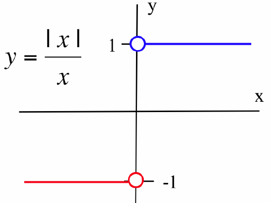
If \(a > 0\), then \(\displaystyle \lim_{x\to a} \, \frac{\left| x \right|}{x} = 1 = f(a)\) so \(f\) is continuous at \(a\).
If \(a < 0\), then \(\displaystyle \lim_{x\to a} \, \frac{\left| x \right|}{x} = -1 = f(a)\) so \(f\) is continuous at \(a\).
But \(f(0)\) is not defined and\[\lim_{x\to 0^{-}} \, \frac{\left| x \right|}{x} = -1 \neq 1 = \lim_{x\to 0^{+}} \, \frac{\left| x \right|}{x}\nonumber\]so \(\displaystyle \lim_{x\to a} \, \frac{\left| x \right|}{x}\) does not exist.
Why Do We Care Whether a Function Is Continuous?
There are several reasons for us to examine continuous functions and their properties:
- Many applications in engineering, the sciences and business are continuous or are modeled by continuous functions or by pieces of continuous functions.
- Continuous functions share a number of useful properties that do not necessarily hold true if the function is not continuous. If a result is true of all continuous functions and we have a continuous function, then the result is true for our function. This can save us from having to show, one by one, that each result is true for each particular function we use. Some of these properties are given in the remainder of this section.
- Differential calculus has been called the study of continuous change, and many of the results of calculus are guaranteed to be true only for continuous functions. If you look ahead into Chapters 2 and 3, you will see that many of the theorems have the form “If \(f\) is continuous and (some additional hypothesis), then (some conclusion).”
Combinations of Continuous Functions
Not only are most of the basic functions we will encounter continuous at most points, so are basic combinations of those functions.
If: \(f(x)\) and \(g(x)\) are continuous at \(a\)
and: \(k\) is any constant
then: the elementary combinations of \(f\) and \(g\)
- \(k\cdot f(x)\)
- \(f(x)+g(x)\)
- \(f(x)-g(x)\)
- \(f(x)\cdot g(x)\)
- \(\displaystyle \frac{f(x)}{g(x)}\) (as long as \(g(a) \neq 0\))
The continuity of a function is defined using limits, and all of these results about simple combinations of continuous functions follow from the results about combinations of limits in the Main Limit Theorem.
Our hypothesis is that \(f\) and \(g\) are both continuous at \(a\), so we can assume that\[\lim_{x\to a} \, f(x) = f(a) \qquad \mbox{and} \qquad \lim_{x\to a} \, g(x) = g(a)\nonumber\]and then use the appropriate part of the Main Limit Theorem.
For example,\[\lim_{x\to a} \, \left[f(x)+g(x)\right] = \lim_{x\to a} \, f(x) + \lim_{x\to a} \, g(x) = f(a) + g(a)\nonumber\]so \(f + g\) is continuous at \(a\).
Prove: If \(f\) and \(g\) are continuous at \(a\), then \(k\cdot f\) and \(f - g\) are continuous at \(a\) (where \(k\) a constant).
- Answer
-
- To prove that \(k\cdot f\) is continuous at \(a\), we need to prove that \(k\cdot f\) satisfies the definition of continuity at \(a\): \(\displaystyle \lim_{x\to a} \, k\cdot f(x) = k\cdot f(a)\). Using results about limits, we know\[\lim_{x\to a} \, k\cdot f(x) = k\cdot \lim_{x\to a} \, f(x) = k\cdot f(a)\nonumber\](because \(f\) is continuous at \(a\)) so \(k\cdot f\) is continuous at \(a\).
- To prove that \(f - g\) is continuous at \(a\), we need to prove that \(f - g\) satisfies the definition of continuity at \(a\): \(\displaystyle \lim_{x\to a} \, \left[f(x)-g(x)\right] = f(a)-g(a)\). Again using information about limits:\[\lim_{x\to a} \, \left[f(x)-g(x)\right] = \lim_{x\to a} \, f(x) - \lim_{x\to a} \, g(x) = f(a)-g(a)\nonumber\](because \(f\) and \(g\) are both continuous at \(a\)) so \(f - g\) is continuous at \(a\).
If: \(g(x)\) is continuous at \(a\)
and: \(f(x)\) is continuous at \(g(a)\)
then: \(\displaystyle \lim_{x\to a} \, f(g(x)) = f(\lim_{x \to a} \, g(x)) = f(g(a))\)
so: \(f\circ g(x) = f( g(x) )\) is continuous at \(a\).
The proof of this result involves some technical details, but just formalizes the following line of reasoning:
The hypothesis that “\(g\) is continuous at \(a\)” means that if \(x\) is close to \(a\) then \(g(x)\) will be close to \(g(a)\). Similarly, “\)f\) is continuous at \(g(a)\)” means that if \(g(x)\) is close to \(g(a)\) then \(f( g(x) ) = f\circ g(x)\) will be close to \(f( g(a) ) = f\circ g(a)\). Finally, we can conclude that if \(x\) is close to \(a\), then \(g(x)\) is close to \(g(a)\) so \(f\circ g(x)\) is close to \(f\circ g(a)\) and therefore \(f\circ g\) is continuous at \(x = a\).
The next theorem presents an alternate version of the limit condition for continuity, which we will use occasionally in the future.
\(\displaystyle \lim_{x\to a} \, f(x) = f(a)\) if and only if \(\displaystyle \lim_{h\to 0} \, f(a+h) = f(a)\)
Proof
Let’s define a new variable \(h\) by \(h = x - a\) so that \(x = a + h\):
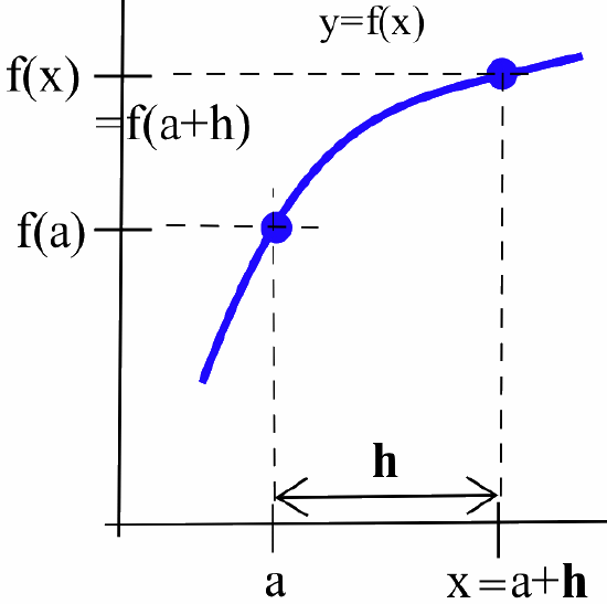
Then \(x \rightarrow a\) if and only if \(h = x - a \rightarrow 0\), so \(\displaystyle \lim_{x\to a} \, f(x) = \lim_{h\to 0} \, f(a+h)\) and therefore \(\displaystyle \lim_{x\to a} \, f(x) = f(a)\) if and only if \(\displaystyle \lim_{h\to 0} \, f(a+h) = f(a)\).
We can restate the result of this theorem as:
A function \(f\) is continuous at \(a\) if and only if \(\displaystyle \lim_{h\to 0} \, f(a+h) = f(a)\).
Which Functions Are Continuous?
Fortunately, the functions we encounter most often are either continuous everywhere or continuous everywhere except at a few places.
The following functions are continuous everywhere
- polynomials
- \(\sin(x)\) and \(\cos(x)\)
- \(\left|x\right|\)
Proof
- This follows from the Substitution Theorem for Polynomial and Rational Functions and the definition of continuity.
- The graph of \(y = \sin(x)\):

clearly has no holes or breaks, so it is reasonable to think that \(\sin(x)\) is continuous everywhere. Justifying this algebraically, recall the angle addition formula for \(\sin(\theta)\) and the results from Section 1.2 that \(\displaystyle \lim_{h\to 0} \, \cos(h) = 1\) and \(\displaystyle \lim_{h\to 0} \, \sin(h) = 0\). For every real number \(a\): \begin{align*} \lim_{h\to 0} \, \sin(a+h) &= \lim_{h\to 0} \, \left[\sin(a)\cos(h) + \cos(a)\sin(h)\right]\\ &= \lim_{h\to 0} \, \sin(a) \cdot \lim_{h\to 0}\, \cos(h) + \lim_{h\to 0} \, \cos(a) \cdot \lim_{h\to 0} \, \sin(h)\\ &= \sin(a) \cdot 1 + \cos(a)\cdot 0 = \sin(a) \end{align*} so \(f(x) = \sin(x)\) is continuous at every point. The justification for \(f(x) = \cos(x)\) is similar. - For \(f(x) = \left|x\right|\), when \(x > 0\), then \(\left|x\right| = x\) and its graph:

is a straight line and is continuous because \(x\) is a polynomial. When \(x <0\), then \(\left|x\right| = -x\) and it is also continuous. The only questionable point is the “corner” on the graph when \(x = 0\), but the graph there is only bent, not broken:\[\lim_{h\to 0^{+}} \, \left|0+h\right| = \lim_{h\to 0^{+}} \, h = 0\nonumber\]and:\[\lim_{h\to 0^{-}} \, \left|0+h\right| = \lim_{h\to 0^{-}} \, -h = 0\nonumber\]so:\[\lim_{h\to 0} \, \left|0+h\right| = 0 = \left|0\right|\nonumber\] and \(f(x) = \left|x\right|\) is also continuous at \(0\).
A continuous function can have corners but not holes or breaks
Even functions that fail to be continuous at some points are often continuous most places:
- A rational function is continuous except where the denominator is \(0\).
- The trig functions \(\tan(x)\), \(\cot(x)\), \(\sec(x)\) and \(\csc(x)\) are continuous except where they are undefined.
- The greatest integer function \(\left\lfloor x \right\rfloor\) is continuous except at each integer.
- But the “holey” function\[h(x) = \left\{ \begin{array}{rl} { 2 } & { \text{if } x \text{ is a rational number }} \\ { 1 } & { \text{if } x \text{ is an irrational number} }\end{array}\right.\nonumber\]is discontinuous everywhere.
Intermediate Value Property of Continuous Functions
Because the graph of a continuous function is connected and does not have any holes or breaks in it, the values of the function can not “skip” or “jump over” a horizontal line:

If one value of the continuous function is below the line and another value of the function is above the line, then somewhere the graph will cross the line. The next theorem makes this statement more precise. The result seems obvious, but its proof is technically difficult and is not given here.
If: \(f\) is continuous on the interval \(\left[a,b\right]\)
and: \(V\) is any value between \(f(a)\) and \(f(b)\)
then: there is a number \(c\) between \(a\) and \(b\) so that \(f(c) = V\).
(That is, \(f\) actually takes on each intermediate value between \(f(a)\) and \(f(b)\).)
If the graph of \(f\) connects the points \((a, f(a))\) and \((b, f(b))\) and \(V\) is any number between \(f(a)\) and \(f(b)\), then the graph of \(f\) must cross the horizontal line \(y = V\) somewhere between \(x = a\) and \(x = b\).
![A graph of a continuous blue curve defined over the closed interval [a, b]. The curve starts at the point (a, f(a)) and ends at (b, f(b)). A horizontal dashed line at height V intersects the curve at a point (c, V), where f(c) = V, illustrating the Intermediate Value Theorem.](https://math.libretexts.org/@api/deki/files/140053/fig103_9.png?revision=1&size=bestfit&width=334&height=285)
Since \(f\) is continuous, its graph cannot “hop” over the line \(y = V\).
We often take this theorem for granted in some common situations:
- If a child’s temperature rose from \(98.6^{\circ}\)F to \(101.3^{\circ}\)F, then there was an instant when the child’s temperature was exactly \(100^{\circ}\)F. (In fact, every temperature between \(98.6^{\circ}\)F and \(101.3^{\circ}\)F occurred at some instant.)
- If you dove to pick up a shell \(25\) feet below the surface of a lagoon, then at some instant in time you were \(17\) feet below the surface. (Actually, you want to be at \(17\) feet twice. Why?)
- If you started driving from a stop (velocity \(= 0\)) and accelerated to a velocity of \(30\) kilometers per hour, then there was an instant when your velocity was exactly \(10\) kilometers per hour.
But we cannot apply the Intermediate Value Theorem if the function is not continuous:
- In 1987 it cost 22¢ to mail a first-class letter inside the United States, and in 1990 it cost 25¢ to mail the same letter, but we cannot conclude that there was a time when it cost 23¢ or 24¢ or ¢ to send the letter. (Postal rates did not increase in a continuous fashion. They jumped directly from 22¢ to 25¢.)
- Prices, taxes and rates of pay change in jumps — discrete steps — without taking on the intermediate values.
The Intermediate Value Theorem (IVT) is an example of an “existence theorem”: it concludes that something exists (a number \(c\) so that \(f(c) = V\)). But like many existence theorems, it does not tell us how to find the the thing that exists (the value of \(c\)) and is of no use in actually finding those numbers or objects.
Bisection Algorithm for Approximating Roots
The IVT can help us finds roots of functions and solve equations. If \(f\) is continuous on \(\left[a,b\right]\) and \(f(a)\) and \(f(b)\) have opposite signs (one is positive and one is negative), then \(0\) is an intermediate value between \(f(a)\) and \(f(b)\) so \(f\) will have a root \(c\) between \(x = a\) and \(x= b\) where \(f(c)= 0\).
While the IVT does not tell us how to find \(c\), it lays the groundwork for a method commonly used to approximate the roots of continuous functions.
Bisection Algorithm for Finding a Root of \(f(x)\)
- Find two values of \(x\) (call them \(a\) and \(b\)) so that \(f(a)\) and \(f(b)\) have opposite signs. (The IVT will then guarantee that \(f(x)\) has a root between \(a\) and \(b\).)
- Calculate the midpoint (or bisection point) of the interval \(\left[a,b\right]\), using the formula \(\displaystyle m = \frac{a+b}{2}\), and evaluate \(f(m)\).
-
- If \(f(m) = 0\), then \(m\) is a root of \(f\) and we are done.
- If \(f(m) \neq 0\), then \(f(m)\) has the sign opposite \(f(a)\) or \(f(b)\):
- if \(f(a)\) and \(f(m)\) have opposite signs, then \(f\) has a root in \(\left[a,m\right]\) so put \(b = m\)
- if \(f(b)\) and \(f(m)\) have opposite signs, then \(f\) has a root in \(\left[m,b\right]\) so put \(a = m\)
- Repeat steps 2 and 3 until a root is found exactly or is approximated closely enough.
The length of the interval known to contain a root is cut in half each time through steps 2 and 3, so the Bisection Algorithm quickly “squeezes” in on a root (see margin figure).
![A graph illustrating the Bisection Method, based on the Intermediate Value Theorem. The blue curve is defined over the first interval [a, b]. Subsequent intervals, such as 'second [M1, b]' and '[M1, M2]' and '[M3, M2]', are progressively smaller, highlighting how the method iteratively narrows down the location of the root.](https://math.libretexts.org/@api/deki/files/140057/fig103_10.png?revision=1&size=bestfit&width=408&height=310)
The steps of the Bisection Algorithm can be done “by hand,” but it is tedious to do very many of them that way. Computers are very good with this type of tedious repetition, and the algorithm is simple to program.
Find a root of \(f(x) = - x^3 + x + 1\).
Solution
\(f(0) = 1\) and \(f(1) = 1\) so we cannot conclude that \(f\) has a root between \(0\) and \(1\). \(f(1) = 1\) and \(f(2) = -5\) have opposite signs, so by the IVT (this function is a polynomial, so it is continuous everywhere and the IVT applies) we know that there is a number \(c\) between \(1\) and \(2\) such that \(f(c) = 0\):
![A graph of the function y = x - x^3 + 1, a smooth blue curve. The graph shows the iterative process of the Bisection Method over the interval [1, 2]. The initial interval is labeled 'first interval', and subsequent narrowed intervals are labeled 'second' and 'third', all leading to the root which is indicated near x = 1.3247.](https://math.libretexts.org/@api/deki/files/140058/fig103_11.png?revision=1&size=bestfit&width=431&height=318)
The midpoint of the interval \(\left[1,2\right]\) is \(m = \frac{1+2}{2} = \frac32 = 1.5\) and \(f(\frac32) = -\frac78\) so \(f\) changes sign between \(1\) and \(1.5\) and we can be sure that there is a root between \(1\) and \(1.5\). If we repeat the operation for the interval \(\left[1, 1.5\right]\), the midpoint is \(m = \frac{1+1.5}{2} = 1.25\), and \(f(1.25) = \frac{19}{64} > 0\) so \(f\) changes sign between \(1.25\) and \(1.5\) and we know \(f\) has a root between \(1.25\) and \(1.5\).
Repeating this procedure a few more times, we get:
| \(a\) | \(b\) | \(m = \frac{b+a}{2}\) | \(f(a)\) | \(f(b)\) | \(f(m)\) | root between | |
|---|---|---|---|---|---|---|---|
| \(1\) | \(2\) | \(1\) | \(-5\) | \(1 | \(2\) | ||
| \(1\) | \(2\) | \(1.5\) | \(1\) | \(-5\) | \(-0.875\) | \(1 | \(1.5\) |
| \(1\) | \(1.5\) | \(1.25\) | \(1\) | \(-0.875\) | \(0.2969\) | \(1.25 | \(1.5\) |
| \(1.25\) | \(1.5\) | \(1.375\) | \(0.2969\) | \(-0.875\) | \(-0.2246\) | \(1.25 | \(1.375\) |
| \(1.25\) | \(1.375\) | \(1.3125\) | \(0.2969\) | \(-0.2246\) | \(0.0515\) | \(1.3125 | \(1.375\) |
| \(1.3125\) | \(1.375\) | \(1.34375\) | |||||
If we continue the table, the interval containing the root will squeeze around the value \(1.324718\).
The Bisection Algorithm has one major drawback: there are some roots it does not find. The algorithm requires that the function take on both positive and negative values near the root so that the graph actually crosses the \(x\)-axis. The function \(f(x) = x^2 - 6x + 9 = (x - 3)^2\) has the root \(x = 3\) but is never negative:
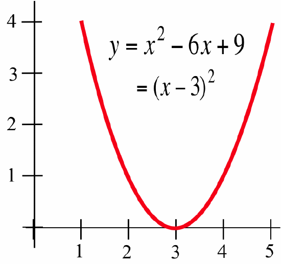
We cannot find two starting points \(a\) and \(b\) so that \(f(a)\) and \(f(b)\) have opposite signs, so we cannot use the Bisection Algorithm to find the root \(x = 3\). In Chapter 2 we will see another method — Newton's Method — that does find roots of this type.
The Bisection Algorithm requires that we supply two starting \(x\)-values, \(a\) and \(b\), at which the function has opposite signs. These values can often be found with a little “trial and error,” or we can examine the graph of the function to help pick the two values.
Finally, the Bisection Algorithm can also be used to solve equations, because the solution of any equation can always be transformed into an equivalent problem of finding roots by moving everything to one side of the equal sign. For example, the problem of solving the equation \(x^3 = x + 1\) can be transformed into the equivalent problem of solving \(x^3 -x -1 = 0\) or of finding the roots of \(f(x) = x^3-x-1\), which is equivalent to the problem we solved in the previous example.
Find all solutions of \(\displaystyle \sin(x) = \frac{2x +1}{x - 2}\) (with \(x\) in radians.)
Solution
We can convert this problem of solving an equation to the problem of finding the roots of\[f(x) = \sin(x) - \frac{2x +1}{x - 2} = 0\nonumber\]The function \(f(x)\) is continuous everywhere except at \(x = 2\), and the graph of \(f(x)\):

can help us find two starting values for the Bisection Algorithm. The graph shows that \(f(-1)\) is negative and \(f(0)\) is positive, and we know \(f(x)\) is continuous on the interval \(\left[-1,0\right]\). Using the algorithm with the starting interval \(\left[-1,0\right]\), we know that a root is contained in the shrinking intervals \(\left[-0.5,0\right]\), \(\left[-0.25,0\right]\), \(\left[-0.25, -0.125\right]\), … , \(\left[-0.238281, -0.236328\right]\), … , \(\left[-0.237176, -0.237177\right]\) so the root is approximately \(-0.237177\).
We might notice that \(f(0) = 0.5>0\) while \(f(\pi) = 0 - \frac{2\pi + 1}{\pi - 2} \approx -6.38 <0\). Why is it wrong to conclude that \(f(x)\) has another root between \(x = 0\) and \(x = \pi\)?
Problems
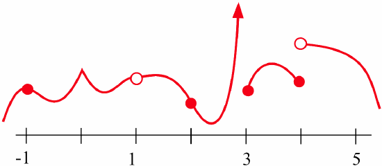
- At which points is the function in the graph below discontinuous?
- At which points is the function in the graph below discontinuous?

- Find at least one point at which each function is not continuous and state which of the three conditions in the definition of continuity is violated at that point.
- \(\displaystyle \frac{x+5}{x-3}\)
- \(\displaystyle \frac{x^2+x-6}{x-2}\)
- \(\displaystyle \sqrt{\cos(x)}\)
- \(\displaystyle \left\lfloor x^2 \right\rfloor\)
- \(\displaystyle \frac{x}{\sin(x)}\)
- \(\displaystyle \frac{x}{x}\)
- \(\displaystyle \ln(x^2)\)
- \(\displaystyle \frac{\pi}{x^2-6x+9}\)
- \(\displaystyle \tan(x)\)
- Which two of the following functions are not continuous? Use appropriate theorems from this section to justify that each of the other functions is continuous.
- \(\displaystyle \frac{7}{\sqrt{2+\sin(x)}}\)
- \(\displaystyle \cos^2(x^5-7x+\pi)\)
- \(\displaystyle \frac{x^2-5}{1+\cos^2(x)}\)
- \(\displaystyle \frac{x^2-5}{1+\cos(x)}\)
- \(\displaystyle \left\lfloor 3+0.5\sin(x) \right\rfloor\)
- \(\displaystyle \left\lfloor 0.3\sin(x) +1.5 \right\rfloor\)
- \(\displaystyle \sqrt{\cos(\sin(x))}\)
- \(\displaystyle \sqrt{x^2-6x+10}\)
- \(\displaystyle \sqrt[3]{\cos(x)}\)
- \(\displaystyle 2^{\sin(x)}\)
- \(\displaystyle 1-3^{-x}\)
- \(\displaystyle \arctan(1-x^2)\)
- A continuous function \(f\) has the values:
\(x\) \(0\) \(1\) \(2\) \(3\) \(4\) \(5\) \(f(x)\) \(5\) \(3\) \(-2\) \(-1\) \(3\) \(-2\) - \(f\) has at least roots between \(0\) and \(5\).
- \(f(x) = 4\) in at least places between \(x = 0\) and \(x = 5\).
- \(f(x) = 2\) in at least places between \(x = 0\) and \(x = 5\).
- \(f(x) = 3\) in at least places between \(x = 0\) and \(x = 5\).
- Is it possible for \(f(x)\) to equal \(7\) for some \(x\)-value(s) between \(0\) and \(5\)?
- A continuous function \(g\) has the values:
\(x\) \(1\) \(2\) \(3\) \(4\) \(5\) \(6\) \(7\) \(g(x)\) \(-3\) \(1\) \(4\) \(-1\) \(3\) \(-2\) \(-1\) - \(g\) has at least roots between \(1\) and \(5\).
- \(g(x) = 3.2\) in at least places between \(x = 1\) and \(x = 7\).
- \(g(x) = -0.7\) in at least places between \(x = 3\) and \(x = 7\).
- \(g(x) = 1.3\) in at least places between \(x = 2\) and \(x = 6\).
- Is it possible for \(g(x)\) to equal \(\pi\) for some \(x\)-value(s) between \(5\) and \(6\)?
- This problem asks you to verify that the Intermediate Value Theorem is true for some particular functions, intervals and intermediate values. In each problem you are given a function \(f\), an interval \(\left[a,b\right]\) and a value \(V\). Verify that \(V\) is between \(f(a)\) and \(f(b)\) and find a value of \(c\) in the given interval so that \(f(c) = V\).
- \(f(x) = x^2\) on \(\left[0,3\right]\), \(V = 2\)
- \(f(x) = x^2\) on \(\left[-1,2\right]\), \(V = 3\)
- \(f(x) = \sin(x)\) on \(\left[0,\frac{\pi}{2}\right]\), \(V = \frac12\)
- \(f(x) = x\) on \(\left[0,1\right]\), \(V = \frac13\)
- \(f(x) = x^2-x\) on \(\left[2,5\right]\), \(V = 4\)
- \(f(x) = \ln(x)\) on \(\left[1,10\right]\), \(V = 2\)
- Two students claim that they both started with the points \(x = 1\) and \(x = 9\) and applied the Bisection Algorithm to the function graphed below:
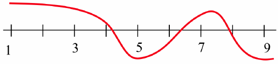
The first student says that the algorithm converged to the root near \(x = 8\), but the second claims that the algorithm will converge to the root near \(x = 4\). Who is correct? - Two students claim that they both started with the points \(x = 0\) and \(x = 5\) and applied the Bisection Algorithm to the function graphed below:

The first student says that the algorithm converged to the root labeled \(A\), but the second claims that the algorithm will converge to the root labeled \(B\). Who is correct? - If you apply the Bisection Algorithm to the function graphed below:

which root does the algorithm find if you use:- starting points \(0\) and \(9\)?
- starting points \(1\) and \(5\)?
- starting points \(3\) and \(5\)?
- If you apply the Bisection Algorithm to the function graphed below:

which root does the algorithm find if you use:- starting points \(3\) and \(7\)?
- starting points \(5\) and \(6\)?
- starting points \(1\) and \(6\)?
In Problems 12–17, use the IVT to verify each function has a root in the given interval(s). Then use the Bisection Algorithm to narrow the location of that root to an interval of length less than or equal to \(0.1\).
- \(f(x) = x^2 - 2\) on \(\left[0, 3\right]\)
- \(g(x) = x^3 - 3x^2 + 3\) on \(\left[-1, 0\right]\), \(\left[1, 2\right]\), \(\left[2,4\right]\)
- \(h(t) = t^5 - 3t + 1\) on \(\left[1, 3\right]\)
- \(r(x) = 5 - 2^x\) on \(\left[1, 3\right]\)
- \(s(x) = \sin(2x) - \cos(x)\) on \(\left[0,\pi\right]\)
- \(p(t) = t^3 + 3t + 1\) on \(\left[-1,1\right]\)
- Explain what is wrong with this reasoning: If \(f(x) = \frac{1}{x}\) then\[f(-1) = -1 < 0 \quad \mbox{and} \quad f(1) = 1 > 0\nonumber\]so \(f\) must have a root between \(x = -1\) and \(x = 1\).
- Each of the following statements is false for some functions. For each statement, sketch the graph of a counterexample.
- If \(f(3) = 5\) and \(f(7) = -3\), then \(f\) has a root between \(x = 3\) and \(x = 7\).
- If \(f\) has a root between \(x = 2\) and \(x = 5\), then \(f(2)\) and \(f(5)\) have opposite signs.
- If the graph of a function has a sharp corner, then the function is not continuous there.
- Define \(A(x)\) to be the area bounded by the \(t\)- and \(y\)-axes, the curve \(y = f(t)\), and the vertical line \(t = x\) as shown in the figure:

It is clear that \(A(1) < 2\) and \(A(3) > 2\). Do you think there is avalue of \(x\) between \(1\) and \(3\) so that \(A(x) = 2\)? If so, justify your conclusion and estimate the location of the value of \(x\) that makes \(A(x) = 2\). If not, justify your conclusion. - Define \(A(x)\) to be the area bounded by the \(t\)- and \(y\)-axes, the curve \(y = f(t)\), and the vertical line \(t = x\) as shown in the figure:

- Shade the part of the graph represented by \(A(2.1) - A(2)\) and estimate the value of \(\displaystyle \frac{A(2.1) - A(2)}{0.1}\).
- Shade the part of the graph represented by \(A(4.1) - A(4)\) and estimate the value of \(\displaystyle \frac{A(4.1) - A(4)}{0.1}\).
-
- A square sheet of paper has a straight line drawn on it from the lower-left corner to the upper-right corner. Is it possible for you to start on the left edge of the sheet and draw a “connected” line to the right edge that does not cross the diagonal line?
- Prove: If \(f\) is continuous on the interval \(\left[0,1\right]\) and \(0 \leq f(x) \leq 1\) for all \(x\), then there is a number \(c\) with \(0 \leq c \leq 1\) such that \(f(c) = c\). (The number \(c\) is called a “fixed point” of \(f\) because the image of \(c\) is the same as \(c\): \(f\) does not “move” \(c\).) Hint: Define a new function \(g(x) = f(x) - x\) and start by considering the values \(g(0)\) and \(g(1)\).
- What does part (b) have to do with part (a)?
- Is the theorem in part (b) true if we replace the closed interval \(\left[0,1\right]\) with the open interval \((0,1)\)?
- A piece of string is tied in a loop and tossed onto quadrant I enclosing a single region:

- Is it always possible to find a line \(L\) passing through the origin so that \(L\) divides the region into two equal areas? (Justify your answer.)
- Is it always possible to find a line \(L\) parallel to the \(x\)-axis so that \(L\) divides the region into two equal areas? (Justify your answer.)
- Is it always possible to find two lines, \(L\) parallel to the \(x\)-axis and \(M\) parallel to the \(y\)-axis, so that \(L\) and \(M\) divide the region into four equal areas? (Justify your answer.)