2.0: Introduction to Derivatives

Last updated
Save as PDF

Page ID: 212010

$ \newcommand{\vecs}[1]{\overset { \scriptstyle \rightharpoonup} {\mathbf{#1}} } $

$ \newcommand{\vecd}[1]{\overset{-\!-\!\rightharpoonup}{\vphantom{a}\smash {#1}}} $

$ \newcommand{\dsum}{\displaystyle\sum\limits} $

$ \newcommand{\dint}{\displaystyle\int\limits} $

$ \newcommand{\dlim}{\displaystyle\lim\limits} $

$ \newcommand{\id}{\mathrm{id}}$ $ \newcommand{\Span}{\mathrm{span}}$

( \newcommand{\kernel}{\mathrm{null}\,}\) $ \newcommand{\range}{\mathrm{range}\,}$

$ \newcommand{\RealPart}{\mathrm{Re}}$ $ \newcommand{\ImaginaryPart}{\mathrm{Im}}$

$ \newcommand{\Argument}{\mathrm{Arg}}$ $ \newcommand{\norm}[1]{\| #1 \|}$

$ \newcommand{\inner}[2]{\langle #1, #2 \rangle}$

$ \newcommand{\Span}{\mathrm{span}}$

$ \newcommand{\id}{\mathrm{id}}$

$ \newcommand{\Span}{\mathrm{span}}$

$ \newcommand{\kernel}{\mathrm{null}\,}$

$ \newcommand{\range}{\mathrm{range}\,}$

$ \newcommand{\RealPart}{\mathrm{Re}}$

$ \newcommand{\ImaginaryPart}{\mathrm{Im}}$

$ \newcommand{\Argument}{\mathrm{Arg}}$

$ \newcommand{\norm}[1]{\| #1 \|}$

$ \newcommand{\inner}[2]{\langle #1, #2 \rangle}$

$ \newcommand{\Span}{\mathrm{span}}$ $ \newcommand{\AA}{\unicode[.8,0]{x212B}}$

$ \newcommand{\vectorA}[1]{\vec{#1}} % arrow$

$ \newcommand{\vectorAt}[1]{\vec{\text{#1}}} % arrow$

$ \newcommand{\vectorB}[1]{\overset { \scriptstyle \rightharpoonup} {\mathbf{#1}} } $

$ \newcommand{\vectorC}[1]{\textbf{#1}} $

$ \newcommand{\vectorD}[1]{\overrightarrow{#1}} $

$ \newcommand{\vectorDt}[1]{\overrightarrow{\text{#1}}} $

$ \newcommand{\vectE}[1]{\overset{-\!-\!\rightharpoonup}{\vphantom{a}\smash{\mathbf {#1}}}} $

$ \newcommand{\vecs}[1]{\overset { \scriptstyle \rightharpoonup} {\mathbf{#1}} } $

$ \newcommand{\vecd}[1]{\overset{-\!-\!\rightharpoonup}{\vphantom{a}\smash {#1}}} $

$\newcommand{\avec}{\mathbf a}$ $\newcommand{\bvec}{\mathbf b}$ $\newcommand{\cvec}{\mathbf c}$ $\newcommand{\dvec}{\mathbf d}$ $\newcommand{\dtil}{\widetilde{\mathbf d}}$ $\newcommand{\evec}{\mathbf e}$ $\newcommand{\fvec}{\mathbf f}$ $\newcommand{\nvec}{\mathbf n}$ $\newcommand{\pvec}{\mathbf p}$ $\newcommand{\qvec}{\mathbf q}$ $\newcommand{\svec}{\mathbf s}$ $\newcommand{\tvec}{\mathbf t}$ $\newcommand{\uvec}{\mathbf u}$ $\newcommand{\vvec}{\mathbf v}$ $\newcommand{\wvec}{\mathbf w}$ $\newcommand{\xvec}{\mathbf x}$ $\newcommand{\yvec}{\mathbf y}$ $\newcommand{\zvec}{\mathbf z}$ $\newcommand{\rvec}{\mathbf r}$ $\newcommand{\mvec}{\mathbf m}$ $\newcommand{\zerovec}{\mathbf 0}$ $\newcommand{\onevec}{\mathbf 1}$ $\newcommand{\real}{\mathbb R}$ $\newcommand{\twovec}[2]{\left[\begin{array}{r}#1 \\ #2 \end{array}\right]}$ $\newcommand{\ctwovec}[2]{\left[\begin{array}{c}#1 \\ #2 \end{array}\right]}$ $\newcommand{\threevec}[3]{\left[\begin{array}{r}#1 \\ #2 \\ #3 \end{array}\right]}$ $\newcommand{\cthreevec}[3]{\left[\begin{array}{c}#1 \\ #2 \\ #3 \end{array}\right]}$ $\newcommand{\fourvec}[4]{\left[\begin{array}{r}#1 \\ #2 \\ #3 \\ #4 \end{array}\right]}$ $\newcommand{\cfourvec}[4]{\left[\begin{array}{c}#1 \\ #2 \\ #3 \\ #4 \end{array}\right]}$ $\newcommand{\fivevec}[5]{\left[\begin{array}{r}#1 \\ #2 \\ #3 \\ #4 \\ #5 \\ \end{array}\right]}$ $\newcommand{\cfivevec}[5]{\left[\begin{array}{c}#1 \\ #2 \\ #3 \\ #4 \\ #5 \\ \end{array}\right]}$ $\newcommand{\mattwo}[4]{\left[\begin{array}{rr}#1 \amp #2 \\ #3 \amp #4 \\ \end{array}\right]}$ $\newcommand{\laspan}[1]{\text{Span}\{#1\}}$ $\newcommand{\bcal}{\cal B}$ $\newcommand{\ccal}{\cal C}$ $\newcommand{\scal}{\cal S}$ $\newcommand{\wcal}{\cal W}$ $\newcommand{\ecal}{\cal E}$ $\newcommand{\coords}[2]{\left\{#1\right\}_{#2}}$ $\newcommand{\gray}[1]{\color{gray}{#1}}$ $\newcommand{\lgray}[1]{\color{lightgray}{#1}}$ $\newcommand{\rank}{\operatorname{rank}}$ $\newcommand{\row}{\text{Row}}$ $\newcommand{\col}{\text{Col}}$ $\renewcommand{\row}{\text{Row}}$ $\newcommand{\nul}{\text{Nul}}$ $\newcommand{\var}{\text{Var}}$ $\newcommand{\corr}{\text{corr}}$ $\newcommand{\len}[1]{\left|#1\right|}$ $\newcommand{\bbar}{\overline{\bvec}}$ $\newcommand{\bhat}{\widehat{\bvec}}$ $\newcommand{\bperp}{\bvec^\perp}$ $\newcommand{\xhat}{\widehat{\xvec}}$ $\newcommand{\vhat}{\widehat{\vvec}}$ $\newcommand{\uhat}{\widehat{\uvec}}$ $\newcommand{\what}{\widehat{\wvec}}$ $\newcommand{\Sighat}{\widehat{\Sigma}}$ $\newcommand{\lt}{<}$ $\newcommand{\gt}{>}$ $\newcommand{\amp}{&}$ $\definecolor{fillinmathshade}{gray}{0.9}$

This section begins with a very graphical approach to slopes of tangent lines. It then examines the problem of finding the slopes of the tangent lines for a single function, $y = x^2$, in some detail — and illustrates how these slopes can help us solve fairly sophisticated problems.

Slopes of Tangent Lines: Graphically

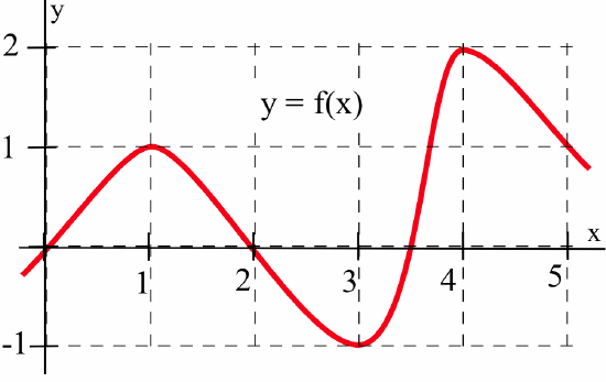
The figure below shows the graph of a function $y = f(x)$.

$A blue wavy line representing the function y = f(x) is plotted on a grid from x = 0 to x = 5. Several short red line segments are drawn tangent to the blue curve at various points to illustrate the slope. These red segments appear at the first peak around x = 1 (where the segment is horizontal), on the downward slope near x = 2, at the bottom of the valley near x = 3 (horizontal), and on the steep upward slope between x = 3 and x = 5.$

We can use the information in the graph to fill in the table:

$x$	$y = f(x)$	$m(x)$
$0$	$0$	$1$
$1$	$1$	$0$
$2$	$0$	$-1$
$3$	$-1$	$0$
$4$	$1$	$1$
$5$	$2$	$\frac12$

where $m(x)$ is the (estimated) slope of the line tangent to the graph of $y=f(x)$ at the point $(x,y)$. We can estimate the values of $m(x)$ at some non-integer values of $x$ as well: $m(0.5) \approx 0.5$ and $m(1.3) \approx -0.3$, for example. We can even say something about the behavior of $m(x)$ over entire intervals: if $0 < x < 1$, then $m(x)$ is positive, for example.

The values of $m(x)$ definitely depend on the values of $x$ (the slope varies as $x$ varies, and there is at most one slope associated with each value of $x$) so $m(x)$ is a function of $x$. We can use the results in the table to help sketch a graph of the function $m(x)$:

$A coordinate graph features a thick red curve labeled m(x) = slope of f(x). The x-axis ranges from 0 to 5, and the y-axis ranges from -1 to 2. The curve begins at y = 1 when x is 0, crosses the x-axis near x = 1.2, reaches a flat bottom at y = -1 between x = 2 and x = 3, and then shoots upward rapidly to a sharp peak of y = 2 around x = 3.6. After the peak, the curve slopes back down toward the x-axis as it moves toward x = 5.$

Practice $\PageIndex{1}$

A graph of $y = f(x)$ appears below. Set up a table of (estimated) values for $x$ and $m(x)$, the slope of the line tangent to the graph of $y=f(x)$ at the point $(x,y)$, and then sketch a graph of the function $m(x)$.

$A blue line graph labeled y = f(x) is plotted on a coordinate grid with an x-axis ranging from 0 to 5 and a y-axis ranging from 0 to 2. The curve starts at y = 2 when x is 0, slopes downward to a local minimum near x = 2, then rises to a local maximum near x = 4 before sloping downward again as it approaches x = 5. Dashed grid lines help indicate the coordinates for various points along the continuous curve.$

Answer

Approximate values of $m(x)$ appear in the table:

$x$	$f(x)$	$m(x)$
$0$	$2$	$-1$
$1$	$1$	$-1$
$2$	$\frac13$	$0$
$3$	$1$	$1$
$4$	$\frac32$	$\frac12$
$5$	$1$	$-2$

The figure shows a graph of $m(x)$ below a graph of $y=f(x)$:

$This image features two vertically stacked graphs. The top graph shows a blue curve labeled y = f(x) on a grid from x = 0 to 5. The curve starts at y = 2, drops to a local minimum near x = 2, and rises to a local maximum near x = 4. The bottom graph is labeled "approximate graph of m(x) = slopes of f(x)" and shows a red curve. This red curve starts near y = -1, stays flat until x = 1.5, rises to cross the x-axis at x = 2, reaches a peak of y = 1 at x = 3, and then falls sharply, crossing the x-axis again near x = 4.2.$

In some applications, we need to know where the graph of a function $f(x)$ has horizontal tangent lines (that is, where the slope of the tangent line equals $0$). The slopes of the lines tangent to graph of $y = f(x)$ in Practice $\PageIndex{1}$ are $0$ when $x = 2$ or $x \approx 4.25$.

Practice $\PageIndex{2}$

At what values of $x$ does the graph of $y = g(x)$ (below) have horizontal tangent lines?

$A horizontal graph shows a single red wavy line labeled y = g(x). The x-axis is marked with integers from -1 to 6. The curve starts above x = -1, dips to a local minimum near x = -0.5, rises to a high peak around x = 1.2, drops to a local minimum near x = 2.8, and rises to a broader, lower peak around x = 5 before starting to trend downward again at x = 6.$

Answer: The tangent lines to the graph of $g$ are horizontal (slope $= 0$) when $x \approx -1$, $1$, $2.5$ and $5$.

Example $\PageIndex{1}$

The graph of the height of a rocket at time $t$ appears below:

$A graph shows the relationship between time and height. The vertical axis is labeled height (feet) with marks at 100, 200, and 300. The horizontal axis is labeled time (seconds) with marks at 5 and 10. A thick blue line starts at the origin (0,0), rises in a smooth curve to a peak of 300 feet at 5 seconds, and then descends. At approximately 8 seconds, the curve changes to a straight downward diagonal line that continues past 10 seconds.$

Sketch a graph of the velocity of the rocket at time $t$. (Remember that instantaneous velocity corresponds to the slope of the line tangent to the graph of position or height function.)

Solution

The top figure below shows some sample tangent line segments:

$This image contains two vertically stacked graphs sharing the same time-axis from 0 to 10 seconds. The top graph shows height in feet with a blue curve reaching a peak of 300 feet at 5 seconds; short red tangent lines are drawn at intervals along this curve. Dashed vertical lines drop down from the peak at 5 seconds and a point of inflection at 8 seconds to the second graph. The bottom graph shows velocity in feet per second with a red line that starts high, crosses zero at 5 seconds, and continues downward until 8 seconds. At 8 seconds, there is a vertical jump to a constant, horizontal red line representing a steady velocity.$

while the bottom figure shows the velocity of the rocket. (What so you think happened at time $t = 8$?)

Practice $\PageIndex{3}$

The graph below shows the temperature during a summer day in Chicago.

$A line graph displays temperature changes over time. The vertical y-axis is labeled temperature (degrees F) with markings at 70, 80, 90, and 100. The horizontal x-axis represents time, with specific labels for 6 AM, noon, and 6 PM. A thick blue line begins at approximately 73 degrees before 6 AM, rises steadily to a peak of about 94 degrees shortly after noon, dips down near 4 PM, rises slightly to a secondary peak around 6 PM, and then begins to drop again.$

Sketch a graph of the rate at which the temperature is changing at each moment in time. (As with instantaneous velocity, the instantaneous rate of change for the temperature corresponds to the slope of the line tangent to the temperature graph.

Answer

The figure below shows a graph of the approximate rate of temperature change (slope) below a graph of the temperature.

$This image contains two vertically stacked graphs relating temperature to time. The top graph shows temperature in degrees Fahrenheit with a blue curve labeled y = f(x); the temperature rises from 6 AM to a peak after noon, dips, and then has a smaller peak at 6 PM. Dashed vertical lines connect the peaks and valleys of the top graph to the bottom graph. The bottom graph, labeled "approximate slopes of f," shows a red curve representing the rate of temperature change in degrees per hour. This red curve stays positive until the first peak, drops to a deep negative valley of -10 at the first dip, and rises to a positive peak before falling again at 6 PM.$

The function $m(x)$, the slope of the line tangent to the graph of $y = f(x)$ at $( x, f(x) )$, is called the derivative of $f(x)$.

We used the idea of the slope of the tangent line all throughout Chapter 1. In Section 2.1, we will formally define the derivative of a function and begin to examine some of its properties, but first let’s see what we can do when we have a formula for $f(x)$.

Tangents to $y = x^2$

When we have a formula for a function, we can determine the slope of the tangent line at a point $( x, f(x) )$:

$A coordinate plane shows a blue curved line labeled y = f(x) and a straight black line labeled secant line that intersects the curve at two blue points. The first point is located at horizontal position x and vertical position f(x), while the second point is further to the right at horizontal position x+h and vertical position f(x+h). Dashed lines extend from these points to the axes to mark their coordinates. A horizontal double-headed arrow between the two points is labeled Run = h, and a vertical double-headed arrow between the two points is labeled Rise = f(x+h) - f(x).$

by calculating the slope of the secant line through the points $( x, f(x) )$ and $( x+h, f(x+h) )$:\[m_{\mbox{sec}} = \frac{f(x+h) - f(x)}{(x+h) - (x)}\]and then taking the limit of $m_{\mbox{sec}}$ as $h$ approaches $0$:\[m_{\mbox{tan}} \ = \ \lim_{h\to 0} \, m_{\mbox{sec}} \ = \ \lim_{h\to 0} \, \frac{f(x+h) - f(x)}{(x+h) - (x)}\]

Example $\PageIndex{2}$

Find the slope of the line tangent to the graph of the function $y = f(x) = x^2$ at the point $(2,4)$.

$A mathematical graph depicts a red curve representing the function y = x^2 starting from the origin (0,0) and curving upward and to the right through the first quadrant. The x-axis is marked with increments of 1 and 2, while the y-axis is marked from 1 to 4. A large red dot is placed on the curve at the coordinate point (2, 4), which is explicitly labeled next to the point.$

Solution

In this example, $x = 2$, so $x + h = 2 + h$ and $f(x + h) = f(2+h) = (2+h)^2$. The slope of the tangent line at $(2,4)$ is \begin{align*} m_{\mbox{tan}} &= \lim_{h\to 0} \, m_{\mbox{sec}} = \lim_{h\to 0} \, \frac{f(2+h) - f(2)}{(2+h) - (2)}\\ &= \lim_{h\to 0} \, \frac{(2+h)^2 - 2^2}{h} = \lim_{h\to 0} \, \frac{4+4h+h^2-4}{h}\\ &= \lim_{h\to 0} \, \frac{4h+h^2}{h} = \lim_{h\to 0} \, [4+h] = 4 \end{align*} The line tangent to $y = x^2$ at the point $(2,4)$ has slope $4$.

We can use the point-slope formula for a line to find an equation of this tangent line:\[y - y_0 = m(x - x_0) \ \Rightarrow \ y - 4 = 4(x - 2) \ \Rightarrow \ y = 4x - 4\nonumber\]

Practice $\PageIndex{4}$

Use the method of Example $\PageIndex{2}$ to show that the slope of the line tangent to the graph of $y = f(x) = x^2$ at the point $(1,1)$ is $m_{\mbox{tan}} = 2$. Also find the values of $m_{\mbox{tan}}$ at $(0,0)$ and $(-1,1)$.

Answer: At $(1,1)$, the slope of the tangent line is:
\begin{align*}
m_{\mbox{tan}} &= \lim_{h\to 0} \, m_{\mbox{sec}} = \lim_{h\to 0} \, \frac{f(1+h) - f(1)}{(1+h) - (1)}\\
&= \lim_{h\to 0} \, \frac{(1+h)^2 - 1^2}{h} = \lim_{h\to 0} \, \frac{1+2h+h^2-1}{h}\\
&= \lim_{h\to 0} \, \frac{2h+h^2}{h} = \lim_{h\to 0} \, [2+h] = 2
\end{align*}
so the line tangent to $y = x^2$ at the point $(1,1)$ has slope $2$. At $(0,0)$:
\begin{align*}
m_{\mbox{tan}} &= \lim_{h\to 0} \, m_{\mbox{sec}} = \lim_{h\to 0} \, \frac{f(0+h) - f(1)}{(0+h) - (0)}\\
&= \lim_{h\to 0} \, \frac{(0+h)^2 - 0^2}{h} = \lim_{h\to 0} \, \frac{h^2}{h} = \lim_{h\to 0} \, h = 0
\end{align*}
so the line tangent to $y = x^2$ at $(0,0)$ has slope $0$. At $(-1,1)$:
\begin{align*}
m_{\mbox{tan}} &= \lim_{h\to 0} \, m_{\mbox{sec}} = \lim_{h\to 0} \, \frac{f(-1+h) - f(-1)}{(-1+h) - (-1)}\\
&= \lim_{h\to 0} \, \frac{(-1+h)^2 - (-1)^2}{h} = \lim_{h\to 0} \, \frac{1-2h+h^2-1}{h}\\
&= \lim_{h\to 0} \, \frac{-2h+h^2}{h} = \lim_{h\to 0} \, [-2+h] = -2
\end{align*}
so the line tangent to $y = x^2$ at the point $(-1,1)$ has slope $-2$.

It is possible to compute the slopes of the tangent lines one point at a time, as we have been doing, but that is not very efficient. You should have noticed in Practice 4 that the algebra for each point was very similar, so let”s do all the work just once, for an arbitrary point $( x, f(x) ) = ( x, x^2 )$ and then use the general result to find the slopes at the particular points we’re interested in.

The slope of the line tangent to the graph of $y = f(x) = x^2$ at the arbitrary point $( x, x^2 )$ is: \begin{align*} m_{\mbox{tan}} &= \lim_{h\to 0} \, m_{\mbox{sec}} = \lim_{h\to 0} \, \frac{f(x+h) - f(x)}{(x+h) - (x)}\\ &= \lim_{h\to 0} \, \frac{(x+h)^2 - x^2}{h} = \lim_{h\to 0} \, \frac{x^2+2xh+h^2-x^2}{h}\\ &= \lim_{h\to 0} \, \frac{2xh+h^2}{h} = \lim_{h\to 0} \, \left[2x+h\right] = 2x \end{align*} The slope of the line tangent to the graph of $y = f(x) = x^2$ at the point $(x, x^2)$ is $m_{\mbox{tan}} = 2x$. We can use this general result at any value of $x$ without going through all of the calculations again. The slope of the line tangent to $y = f(x) = x^2$ at the point $(4, 16)$ is $m_{\mbox{tan}} = 2(4) = 8$ and the slope at $(p, p^2)$ is $m_{\mbox{tan}} = 2(p) = 2p$. The value of $x$ determines the location of our point on the curve, $(x, x^2)$, as well as the slope of the line tangent to the curve at that point, $m_{\mbox{tan}} = 2x$. The slope $m_{\mbox{tan}} = 2x$ is a function of $x$ and is called the derivative of $y = x^2$.

Simply knowing that the slope of the line tangent to the graph of $y = x^2$ is $m_{\mbox{tan}} = 2x$ at a point $(x,y)$ can help us quickly find an equation of the line tangent to the graph of $y = x^2$ at any point and answer a number of difficult-sounding questions.

Example $\PageIndex{3}$

Find equations of the lines tangent to $y = x^2$ at the points $(3, 9)$ and $(p, p^2)$.

Solution

At $(3, 9)$, the slope of the tangent line is $2x = 2(3) = 6$, and the equation of the line is $y - 9 = 6(x - 3) \Rightarrow y = 6x - 9$.

At $(p, p^2)$, the slope of the tangent line is $2x = 2(p) = 2p$, and the equation of the line is $y - p^2 = 2p(x - p) \Rightarrow y = 2px - p^2$.

Example $\PageIndex{4}$

A rocket has been programmed to follow the path $y = x^2$ in space (from left to right along the curve, as seen in the figure below), but an emergency has arisen and the crew must return to their base, which is located at coordinates $(3,5)$.

$A coordinate plane shows a blue curve for the function y = x^2 starting at the origin. A blue point on the curve is labeled (p, q) and is located near x = 1. A second point, colored red, is located off the curve at the coordinate (3, 5). A dashed black line serves as a secant line connecting the blue point (p, q) to the red point (3, 5). The x-axis is marked with 1, 2, and 3, while the y-axis is marked with 2 and 5.$

At what point on the path $y = x^2$ should the captain turn off the engines so that the ship will coast along a path tangent to the curve to return to the base?

Solution

You might spend a few minutes trying to solve this problem without using the relation $m_{\mbox{tan}} = 2x$, but the problem is much easier if we do use that result.

Let’s assume that the captain turns off the engine at the point $(p,q)$ on the curve $y = x^2$ and then try to determine what values $p$ and $q$ must have so that the resulting tangent line to the curve will go through the point $(3,5)$. The point $(p,q)$ is on the curve $y = x^2$, so $q = p^2$ and the equation of the tangent line, found in Example $\PageIndex{3}$, must then be $y = 2px - p^2$.

To find the value of $p$ so that the tangent line will go through the point $(3,5)$, we can substitute the values $x = 3$ and $y = 5$ into the equation of the tangent line and solve for $p$: \begin{align*}y = 2px - p^2 \ \Rightarrow \ 5 = 2p(3) - p^2 \ &\Rightarrow \ p^2 - 6p + 5 = 0\\ &\Rightarrow \ (p - 1)(p - 5) = 0\end{align*} The only solutions are $p = 1$ and $p = 5$, so the only possible points are $(1,1)$ and $(5,25)$.

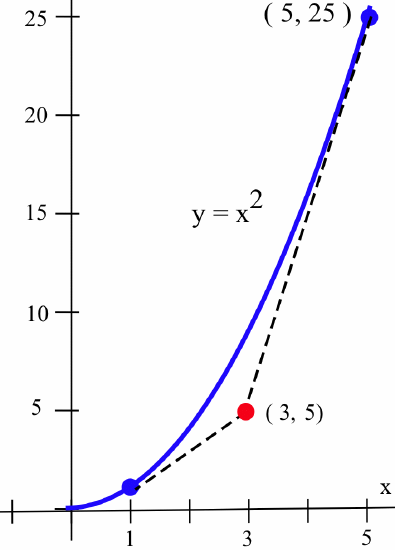
$A mathematical graph depicts a blue curve for the function y = x^2 starting from the origin. Three specific points are highlighted. A blue point is located near the start of the curve at x = 1. A red point is located at the coordinate (3, 5), which sits below the curve. A second blue point is located higher up on the curve at the coordinate (5, 25), which is labeled in the top right. A dashed black secant line connects the blue point at x = 1 to the blue point at (5, 25), passing through the red point at (3, 5).$

You can verify that the tangent lines to $y = x^2$ at $(1,1)$ and $(5,25)$ both go through the point $(3,5)$. Because the ship is moving from left to right along the curve, the captain should turn off the engines at the point $(1,1)$. (Why not at $(5,25)$?)

Practice $\PageIndex{5}$

Verify that if the rocket engines in Example 4 are shut off at $(2,4)$, then the rocket will go through the point $(3,8)$.

Answer: From Example $\PageIndex{4}$ we know the slope of the tangent line is $m_{\mbox{tan}} = 2x$, so the slope of the tangent line at $(2,4)$ is $m_{\mbox{tan}} = 2x = 2(2) = 4$. The tangent line has slope $4$ and goes through the point $(2,4)$, so an equation of the tangent line (using $y - y_0 = m(x - x_0)$) is $y - 4 = 4(x - 2)$ or $y = 4x - 4$. The point $(3,8)$ satisfies the equation $y = 4x - 4$, so the point $(3,8)$ lies on the tangent line.

Problems

Use the function $f(x)$ graphed below to fill in the table and then graph $m(x)$, the estimated slope of the tangent line to $y=f(x)$ at the point $(x,y)$.
$A coordinate graph shows a red curve representing the function y = f(x) on a grid with an x-axis from 0 to 4 and a y-axis from -1 to 2. The curve starts at (0, 1), rises to a rounded peak of approximately y = 1.6 near x = 1.2, and then descends steadily. It crosses the x-axis at approximately x = 2.8 and reaches a local minimum near the bottom right of the grid at x = 3.6 before curving slightly upward at x = 4.$

$x$	$f(x)$	$m(x)$	$x$	$f(x)$	$m(x)$
$0.0$			$2.5$
$0.5$			$3.0$
$1.0$			$3.5$
$1.5$			$4.0$
$2.0$

Use the function $g(x)$ graphed below to fill in the table and then graph $m(x)$, the estimated slope of the tangent line to $y=g(x)$ at the point $(x,y)$.
$A coordinate graph shows a blue curve representing the function y = g(x) on a grid. The x-axis is marked from 1 to 4 and the y-axis from -1 to 2. The curve starts slightly above the x-axis at x = 0.5, dips to a local minimum near x = 1.4, crosses the x-axis at x = 2, and rises to a local maximum of approximately y = 1.4 near x = 3.2 before sloping downward and crossing the x-axis again at x = 4.$

$x$	$g(x)$	$m(x)$	$x$	$g(x)$	$m(x)$
$0.0$			$2.5$
$0.5$			$3.0$
$1.0$			$3.5$
$1.5$			$4.0$
$2.0$

1. At what values of $x$ does the graph of $f$ (shown below) have a horizontal tangent line?
  $A coordinate graph displays a thick red curve representing the function y = f(x). The grid has an x-axis ranging from 0 to 5 and a y-axis from -1 to 2. The curve starts at the origin, rises to a local maximum of y = 1 at x = 1, crosses the x-axis at x = 2, and reaches a local minimum of y = -1 at x = 3. It then shoots upward rapidly to a high peak of nearly y = 2 at x = 4 before sloping downward toward the point (5, 1).$
2. At what value(s) of $x$ is the value of $f$ the largest? Smallest?
3. Sketch a graph of $m(x)$, the slope of the line tangent to the graph of $f$ at the point $(x,f(x))$.
1. At what values of $x$ does the graph of $g$ (shown below) have a horizontal tangent line?
  $A coordinate graph displays a blue curve for the function y = g(x) on a grid where the x-axis is marked 1 through 5 and the y-axis is marked -1 to 2. The curve starts near y = 1.6, descends to a local minimum of y = 0.8 at x = 1.2, and rises sharply to a local maximum of y = 2 at x = 2.2. After the peak, it drops to a second local minimum of y = 1 at x = 3.2 and then follows a steady, shallow upward slope toward the point (5.5, 2).$
2. At what value(s) of $x$ is the value of $g$ the largest? Smallest?
3. Sketch a graph of $m(x)$, the slope of the line tangent to the graph of $g$ at the point $(x,g(x))$.
1. Sketch the graph of $f(x) = \sin(x)$ on the interval $-3 \leq x \leq 10$.
2. Sketch a graph of $m(x)$, the slope of the line tangent to the graph of $\sin(x)$ at the point $(x, \sin(x))$.
3. Your graph in part (b) should look familiar. What function is it?
Match the situation descriptions with the corresponding time-velocity graphs shown below.
1. A car quickly leaving from a stop sign.
2. A car sedately leaving from a stop sign.
3. A student bouncing on a trampoline.
4. A ball thrown straight up.
5. A student confidently striding across campus to take a calculus test.
6. An unprepared student walking across campus to take a calculus test.

Problems 7–10 assume that a rocket is following the path $y = x^2$, from left to right.

At what point should the engine be turned off in order to coast along the tangent line to a base at $(5,16)$?
At $(3,-7)$?
At $(1,3)$?
Which points in the plane can not be reached by the rocket? Why not?

In Problems 11–16, perform these steps:

Calculate and simplify: $\displaystyle m_{\mbox{sec}} = \frac{f(x+h) - f(x)}{(x+h) - (x)}$
Determine $\displaystyle m_{\mbox{tan}} = \lim_{h\to 0} \, m_{\mbox{sec}}$.
Evaluate $m_{\mbox{tan}}$ at $x = 2$.
Find an equation of the line tangent to the graph of $f$ at $(2, f(2))$.

$f(x) = 3x - 7$
$f(x) = 2 - 7x$
$f(x) = ax + b$ where $a$ and $b$ are constants
$f(x) = x^2 + 3x$
$f(x) = 8 - 3x^2$
$f(x) = ax^2 + bx + c$ where $a$, $b$ and $c$ are constants

In Problems 17–18, use the result: $\displaystyle f(x) = ax^2 + bx + c \ \Rightarrow \ m_{\mbox{tan}} = 2ax + b$

Given $f(x) = x^2 + 2x$, at which point(s) $(p, f(p))$ does the line tangent to the graph at that point also go through the point $(3, 6)$?
1. If $a \neq 0$, then what is the shape of the graph of $y = f(x) = ax^2 + bx + c$?
2. At what value(s) of $x$ is the line tangent to the graph of $f(x)$ horizontal?

\(x\)	\(y = f(x)\)	\(m(x)\)
\(0\)	\(0\)	\(1\)
\(1\)	\(1\)	\(0\)
\(2\)	\(0\)	\(-1\)
\(3\)	\(-1\)	\(0\)
\(4\)	\(1\)	\(1\)
\(5\)	\(2\)	\(\frac12\)

\(x\)	\(f(x)\)	\(m(x)\)
\(0\)	\(2\)	\(-1\)
\(1\)	\(1\)	\(-1\)
\(2\)	\(\frac13\)	\(0\)
\(3\)	\(1\)	\(1\)
\(4\)	\(\frac32\)	\(\frac12\)
\(5\)	\(1\)	\(-2\)

\(x\)	\(f(x)\)	\(m(x)\)	\(x\)	\(f(x)\)	\(m(x)\)
\(0.0\)			\(2.5\)
\(0.5\)			\(3.0\)
\(1.0\)			\(3.5\)
\(1.5\)			\(4.0\)
\(2.0\)

\(x\)	\(g(x)\)	\(m(x)\)	\(x\)	\(g(x)\)	\(m(x)\)
\(0.0\)			\(2.5\)
\(0.5\)			\(3.0\)
\(1.0\)			\(3.5\)
\(1.5\)			\(4.0\)
\(2.0\)

Search

Text Color

Text Size

Margin Size

Font Type

Practice \(\PageIndex{1}\)

Practice \(\PageIndex{2}\)

Example \(\PageIndex{1}\)

Solution

Practice \(\PageIndex{3}\)

Example \(\PageIndex{2}\)

Solution

Practice \(\PageIndex{4}\)

Example \(\PageIndex{3}\)

Solution

Example \(\PageIndex{4}\)

Solution

Practice \(\PageIndex{5}\)

Slopes of Tangent Lines: Graphically

Practice \(\PageIndex{1}\)

Practice \(\PageIndex{2}\)

Example \(\PageIndex{1}\)

Solution

Practice \(\PageIndex{3}\)

Tangents to \(y = x^2\)

Example \(\PageIndex{2}\)

Solution

Practice \(\PageIndex{4}\)

Example \(\PageIndex{3}\)

Solution

Example \(\PageIndex{4}\)

Solution

Practice \(\PageIndex{5}\)

Problems