2.1: The Definition of Derivative

The graphical idea of a slope of a tangent line is very useful, but for some purposes we need a more algebraic definition of the derivative of a function. We will use this definition to calculate the derivatives of several functions and see that these results agree with our graphical understanding. We will also look at several different interpretations for the derivative, and obtain a theorem that will allow us to easily and  quickly determine the derivative of any fixed power of \(x\).

In the previous section we found the slope of the tangent line to the graph of the function \(f(x) = x^2\) at an arbitrary point \((x, f(x))\) by calculating the slope of the secant  line through the points \((x, f(x))\) and \((x+h, f(x+h))\):\[m_{\mbox{sec}} = \frac{f(x+h) - f(x)}{(x+h) - (x)}\nonumber\]and then taking the limit of \(m_{\mbox{sec}}\) as \(h\) approached \(0\):

That approach to calculating slopes of tangent lines motivates the definition of the derivative of a function.

Definition of the Derivative

The derivative of a function \(f\) is a new function, \(f'\) (pronounced “eff prime”), whose value at \(x\) is:\[f'(x) = \lim_{h\to 0} \, \frac{f(x+h) - f(x)}{h}\nonumber\]if this limit exists and is finite.

This is the definition of differential calculus, and you must know it and understand what it says. The rest of this chapter and all of Chapter 3 are built on this definition, as is much of what appears in later chapters. It is remarkable that such a simple idea (the slope of a tangent line) and such a simple definition (for the derivative \(f'\)) will lead to so many important ideas and applications.

Notation

There are three commonly used notations for the derivative of \(y = f(x)\):

• \(f'(x)\) emphasizes that the derivative is a function related to \(f\)
• \(\mbox{D}(f)\) emphasizes that we perform an operation on \(f\) to get \(f'\)
• \(\displaystyle \frac{df}{dx}\) emphasizes that the derivative is the limit of \(\displaystyle \frac{\Delta f}{\Delta x} = \frac{f(x+h) - f(x)}{h}\)

We will use all three notations so that you can become accustomed to working with each of them.

The function \(f'(x)\) gives the slope of the tangent line to the graph of \(y = f(x)\) at the point \((x, f(x))\), or the instantaneous rate of change of the function \(f\) at the point \((x, f(x))\).

If, in the figure below, we let \(x\) be the point \(a+h\), then \(h = x - a\):

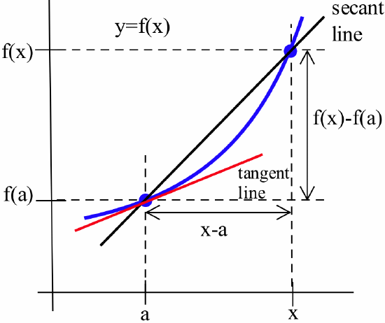
As \(h\rightarrow 0\), we see that \(x\rightarrow a\) and:\[f'(a) = \lim_{h\to 0} \, \frac{f(a+h) - f(a)}{h} = \lim_{x\to a} \, \frac{f(x) - f(a)}{x-a}\nonumber\]

We will use whichever of these two forms is more convenient algebraically in a particular situation.

Calculating Some Derivatives Using the Definition

Fortunately, we will soon have some quick and easy ways to calculate most derivatives, but first we will need to use the definition to determine the derivatives of a few basic functions. In Section 2.2, we will use those results and some properties of derivatives to calculate derivatives of combinations of the basic functions. Let’s begin by using the graphs and then the definition to find a few derivatives.

Example \(\PageIndex{1}\)

Graph \(y = f(x) = 5\) and estimate the {\bf slope} of the tangent line at each point on the graph. Then use the definition of the derivative to calculate the exact slope of the tangent line at each point. Your  graphical estimate and the exact result from the definition should agree.

Solution

The graph of \(y = f(x) = 5\) is a horizontal line, which has slope \(0\), so we should expect that its tangent line will also have slope \(0\).

Using the definition: With \(f(x) = 5\), then \(f(x+h) = 5\) no matter what \(h\) is, so:\[\mbox{D}( f(x) ) = \lim_{h\to 0} \, \frac{f(x+h) - f(x)}{h} = \lim_{h\to 0} \, \frac{5-5}{h} = \lim_{h\to 0} \, 0 = 0\nonumber\]and this agrees with our graphical estimate of the derivative.

Using similar steps, it is easy to show that the derivative of {\em any} constant function is \(0\).

Theorem

If \(f(x) = k\), then \(f'(x) = 0\).

Practice \(\PageIndex{1}\)

Graph \(y = f(x) = 7x\) and estimate the slope of the tangent line at each point on the graph. Then use the definition of the derivative to calculate the exact slope of the tangent line at each point.

Answer

The graph of \(f(x) = 7x\) is a line through the origin. The slope of the line is \(7\). For all \(x\):\[m_{\mbox{tan}} = \lim_{h\to 0} \, \frac{f(x + h) - f(x)}{h} = \lim_{h\to 0} \, \frac{7(x + h) -7x}{h} = \lim_{h\to 0} \, \frac{7h}{h} = \lim_{h\to 0}\, 7 = 7\nonumber\]

Example \(\PageIndex{2}\)

Describe the derivative of \(y = f(x) = 5x^3\) graphically and compute it using the definition. Find an equation of the line tangent to \(y = 5x^3\) at the point \((1,5)\).

Solution

It appears from the graph of \(y = f(x) = 5x^3\) (see margin) that \(f(x)\) is increasing, so the slopes of the tangent lines are positive except perhaps at \(x = 0\), where the graph seems to flatten out.

With \(f(x) = 5x^3\) we have:\[f(x+h) = 5(x+h)^3 = 5(x^3 + 3x^2 h + 3xh^2 + h^3 )\nonumber\]and using this last expression in the definition of the derivative: \begin{align*}f'(x) &= \lim_{h\to 0} \, \frac{f(x+h) - f(x)}{h} = \lim_{h\to 0} \, \frac{5(x^3 + 3x^2 h + 3xh^2 + h^3) - 5x^3}{h}\\ &= \lim_{h\to 0} \, \frac{15x^2 h + 15xh^2 + 5h^3}{h} = \lim_{h\to 0} \, (15x^2 + 15xh + 5h^2) = 15x^2 \end{align*} so \(\mbox{D}(5x^3) = 15x^2\), which is positive except when \(x=0\) (as we predicted from the graph).

The function \(f'(x) = 15x^2\) gives the slope of the line tangent to the graph of \(f(x) = 5x^3\) at the point \((x,f(x))\). At the point \((1,5)\), the slope of the tangent line is \(f'(1) = 15(1)^2 = 15\). From the point-slope formula, an equation of the tangent line to \(f\) at that point is \(y - 5 = 15( x - 1)\) or \(y = 15x - 10\).

Practice \(\PageIndex{2}\)

Use the definition to show that the derivative of \(y = x^3\) is \(\displaystyle \frac{dy}{dx} = 3x^2\). Find an equation of the line tangent to the graph of \(y = x^3\) at the point \((2, 8)\).

Answer

\(f(x) = x^3 \Rightarrow f(x + h) = (x + h)^3 = x^3 + 3x^2h + 3xh^2 + h^3\) so: \begin{align*}f'(x) &= \lim_{h\to 0} \, \frac{f(x + h) - f(x)}{h} = \lim_{h\to 0} \, \frac{x^3 + 3x^2h + 3xh^2 + h^3 - x^3}{h}\\
                    &= \lim_{h\to 0} \, \frac{3x^2h + 3xh^2 + h^3}{h} = \lim_{h\to 0} \, 3x^2 + 3xh + h^2 = 3x^2
\end{align*} At the point \((2,8)\), the slope of the tangent line is \(3(2)^2 = 12\) so an equation of the tangent line is \(y - 8 = 12(x - 2)\) or \(y = 12x -16\).

If \(f\) has a derivative at \(x\), we say that \(f\) is differentiable at \(x\). If we have a point on the graph of a differentiable function and a slope (the derivative evaluated at the point), it is easy to write an equation of the tangent line.

Tangent Line Formula

If: \(f(x)\) is differentiable at \(x=a\)

then: an equation of the line tangent to \(f\) at \((a ,f(a) )\) is:\[y = f(a) + f'(a)(x - a)\nonumber\]

Proof

The tangent line goes through the point \(( a , f(a) )\) with slope \(f'(a)\) so, using the point-slope formula, \(y - f(a) = f '(a) (x - a)\) or \(y = f(a) + f '(a) (x - a)\).

Practice \(\PageIndex{3}\)

The derivatives \(\mbox{D}( x ) = 1\), \(\mbox{D}( x^2 ) = 2x\), \(\mbox{D}( x^3 ) = 3x^2\) exhibit the start of a pattern. Without using the definition of the derivative, what do you think the following derivatives will be? \(\mbox{D}( x^4 )\), \(\mbox{D}( x^5 )\), \(\mbox{D}( x^{43} )\), \(\mbox{D}( \sqrt{x} ) = \mbox{D}( x^{\frac12})\) and \(\mbox{D}( x^{\pi} )\). (Just make an intelligent “guess” based on the pattern of the previous examples.)

Answer

\(\mbox{D}( x^4) = 4x^3\), \(\mbox{D}( x^5) = 5x^4\), \(\mbox{D}( x^{43}) = 43x^{42}\), \(\mbox{D}( \sqrt{x}) = \mbox{D}( x^{\frac12}) = \frac12 x^{-\frac12} = \frac{1}{2\sqrt{x}}\), \(\mbox{D}( x^{\pi}) = \pi x^{\pi -1}\)

Before further investigating the “pattern” for the derivatives of powers of \(x\) and general properties of derivatives, let’s compute the derivatives of two functions that are not powers of \(x\): \(\sin(x)\) and \(\left| x \right|\).

Theorem

\(\mbox{D}( \sin(x) ) = \cos(x)\)

The graph of \(y = f(x) = \sin(x)\) should be very familiar to you:

The graph has horizontal tangent lines (slope \(= 0\)) when \(x = \pm \frac{\pi}{2}\) and \(x = \pm \frac{3\pi}{2}\)  and so on. If \(0 < x < \frac{\pi}{2}\), then the slopes of the tangent lines to the graph of \(y = \sin(x)\) are positive. Similarly, if \(\frac{\pi}{2} < x < \frac{3\pi}{2}\), then the slopes of the tangent lines are negative. Finally, because the graph of \(y = \sin(x)\) is periodic, we expect that the derivative of \(y = \sin(x)\)  will also be periodic. Note that the function \(\cos(x)\) possesses all of those desired properties for the slope function.

Proof

With \(f(x) = \sin(x)\), apply an angle addition formula to get:\[f(x+h) = \sin(x+h) = \sin(x)\cos(h) + \cos(x)\sin(h)\nonumber\]and use this formula in the definition of the derivative:
\begin{align*}
f'(x) &= \lim_{h\to 0} \, \frac{f(x + h) - f(x)}{h}\\
      &= \lim_{h\to 0} \, \frac{\left(\sin(x)\cos(h)+\cos(x)\sin(h)\right)-\sin(x)}{h}\end{align*}
This limit looks formidable, but just collect the terms containing \(\sin(x)\):\[\lim_{h\to 0} \, \frac{\left(\sin(x)\cos(h)-\sin(x)\right)+\cos(x)\sin(h)}{h}\nonumber\]so you can factor out \(\sin(x)\) from the first two terms, rewriting as:
\[\lim_{h\to 0} \, \left[\sin(x)\cdot \frac{\cos(h) - 1}{h} + \cos(x)\cdot \frac{\sin(h)}{h}\right]\nonumber\]Now calculate the limits separately:\[\lim_{h\to 0} \, \sin(x) \cdot \lim_{h\to 0} \, \frac{\cos(h) - 1}{h} + \lim_{h\to 0} \, \cos(x) \cdot \lim_{h\to 0} \, \frac{\sin(h)}{h}\nonumber\]The first and third limits do not depend on \(h\), and we calculated the second and fourth limits in Section 1.2:\[\sin(x)\cdot 0 + \cos(x)\cdot 1 = \cos(x)\nonumber\]So \(\mbox{D}( \sin(x) ) = \cos(x)\) and the various properties we expected of the derivative of \(y = \sin(x)\) by examining its graph are true of \(\cos(x)\).

Practice \(\PageIndex{4}\)

Show that \(\mbox{D}(\cos(x) ) = -\sin(x)\) using the definition.

You will need the angle addition formula for cosine to rewrite \(\cos(x+h)\) as:\[\cos(x)\cdot\cos(h) - \sin(x)\cdot\sin(h)\nonumber\]

Answer

Proceeding as we did to find the derivative to \(\sin(x)\): \begin{align*}\mbox{D}( \cos(x) ) &= \lim_{h\to 0} \, \frac{\cos(x + h) - \cos(x)}{h} = \lim_{h\to 0} \, \frac{\cos(x)\cos(h) - \sin(x)\sin(h) - cos(x)}{h}\\ &= \lim_{h\to 0} \, \left[\cos(x)\cdot \frac{\cos(h) - 1}{h} - \sin(x)\frac{\sin(h)}{h}\right] = \cos(x)\cdot0 - \sin(x)\cdot 1 = -\sin(x) \end{align*}

The derivative of \(\cos(x)\) resembles the situation for \(\sin(x)\) but differs by an important negative sign. You should memorize both of these important derivatives.

Example \(\PageIndex{3}\)

For \(y = \left|x\right|\), find \(\displaystyle \frac{dy}{dx}\).

Solution

The graph of \(y = f(x) = \left| x \right|\) is a “V” shape with its vertex at the origin:

When \(x > 0\), the graph is just \(y = \left|x\right| = x\), which is part of a line with slope \(+1\), so we should expect the derivative of \(\left|x\right|\) to be \(+1\). When \(x < 0\), the graph is \(y = \left|x\right| = -x\), which is part of a line with slope \(-1\), so we expect the derivative of \(\left|x\right|\) to be \(-1\). When \(x = 0\), the graph has a corner, and we should expect the derivative of \(\left|x\right|\) to be undefined at \(x = 0\), as there is no single candidate for a line tangent to the graph there.

Using the definition, consider the same three cases discussed previously: \(x > 0\), \(x < 0\) and \(x = 0\).

If \(x > 0\), then, for small values of \(h\), \(x + h > 0\), so:\[\mbox{D} (f(x)) = \lim_{h\to 0} \, \frac{\left| x + h \right| - \left| x \right|}{h} = \lim_{h\to 0}\, \frac{x+h-x}{h} = \lim_{h\to 0}\, \frac{h}{h} = 1\nonumber\] If \(x < 0\), then, for small values of \(h\), \(x + h < 0\), so:\[\mbox{D} (f(x)) = \lim_{h\to 0} \, \frac{\left| x + h \right| - \left| x \right|}{h} = \lim_{h\to 0}\, \frac{-(x+h)-(-x)}{h} = \lim_{h\to 0}\, \frac{-h}{h} = -1\nonumber\]When \(x = 0\), the situation is a bit more complicated:\[f'(0) = \lim_{h\to 0} \, \frac{\left| 0 + h \right| - \left| 0 \right|}{h} = \lim_{h\to 0}\, \frac{\left|h\right|}{h}\nonumber\]This is undefined, as \(\displaystyle \lim_{h\to 0^{+}} \, \frac{\left|h\right|}{h} = +1\) and \(\displaystyle \lim_{h\to 0^{-}} \, \frac{\left|h\right|}{h} = -1\), so:\[\mbox{D}(\left|x\right|) = \left\{
\begin{array}{rl}
1 & \mbox{if }x > 0\\
\mbox{undefined} & \mbox{if }x=0\\
-1 & \mbox{if }x<0\end{array}\right.\nonumber\]or, equivalently, \(\displaystyle \mbox{D}(\left|x\right|) = \frac{\left|x\right|}{x}\).

The derivative of \(\left|x\right|\) agrees with the function \(\sgn(x)\) defined in Chapter 0, except at \(x=0\): \(\mbox{D}(\left|x\right|)\) is undefined at \(x = 0\) but \(\sgn(0) = 0\).

Practice \(\PageIndex{5}\)

Graph \(y = \left| x - 2 \right|\) and \(y = \left| 2x \right|\) and use the graphs to determine \(\mbox{D}( \left|x - 2\right| )\) and \(\mbox{D}( \left| 2x \right| )\).

Answer

Here are the graphs of \(y = \left| x - 2 \right|\) \(y = \left| 2x \right|\):

 

\begin{align*}\mbox{D}(\left|x-2\right|) &= \left\{
\begin{array}{rl}
{ 1 } & { \text {if } x > 2 } \\
{ \text{undefined} } & { \text{if } x = 2 } \\
{ -1 } & { \text {if } x < 2 } \end{array}\right. \ = \ \frac{\left|x-2\right|}{x-2}\\
\mbox{D}(\left|2x\right|) &= \left\{
\begin{array}{rl}
{ 2 } & { \text{if } x > 0 } \\
{ \mbox{undefined} } & { \text{if } x = 0 } \\
{ -2 } & { \mbox{if } x < 0 } \end{array}\right. \ = \ \frac{2\left|x\right|}{x}
\end{align*}

So far we have emphasized the derivative as the slope of the line tangent to a graph. That very visual interpretation is very useful when examining the graph of a function, and we will continue to use it. Derivatives, however, are employed in a wide variety of fields and applications, and some of these fields use other interpretations. A few commonly used interpretations of the derivative follow.

Interpretations of the Derivative

General

Rate of Change: The function \(f '(x)\) is the rate of change of the function at \(x\). If the units for \(x\) are years and the units for \(f(x)\) are people, then the units for \(\frac{df}{dx}\) are \(\frac{\mbox{people}}{\mbox{year}}\), a rate of change in population.

Graphical

Slope: \(f'(x)\) is the slope of the line tangent to the graph of \(f\) at \(( x, f(x) )\).

Physical

Velocity: If \(f(x)\) is the position of an object at time \(x\), then \(f'(x)\) is the velocity of the object at time \(x\). If the units for \(x\) are hours and \(f(x)\) is distance, measured in miles, then the units for \(f'(x) = \frac{df}{dx}\) are \(\frac{\mbox{miles}}{\mbox{hour}}\), miles per hour, which is a measure of velocity.

Acceleration: If \(f(x)\) is the velocity of an object at time \(x\), then \(f'(x)\) is the acceleration of the object at time \(x\). If the units for \(x\) are hours and \(f(x)\) has the units \(\frac{\mbox{miles}}{\mbox{hour}}\), then the units for the acceleration \(f'(x) = \frac{df}{dx}\) are \(\frac{\mbox{miles/hour}}{\mbox{hour}} = \frac{\mbox{miles}}{\mbox{hour}^2}\), “miles per hour per hour.”

Magnification: \(f'(x)\) is the magnification factor of the function \(f\) for points close to \(x\). If \(a\) and \(b\) are two points very close to \(x\), then the distance between \(f(a)\) and \(f(b)\) will be close to \(f'(x)\) times the original distance between \(a\) and \(b\): \(f(b) - f(a) \approx f'(x) ( b - a )\).

Business

Marginal Cost: If \(f(x)\) is the total cost of producing \(x\) objects, then \(f'(x)\) is the marginal cost, at a production level of \(x\): (approximately) the additional cost of making one more object once we have already made \(x\) objects. If the units for \(x\) are bicycles and the units for \(f(x)\) are dollars, then the units for \(f'(x) = \frac{df}{dx}\) are \(\frac{\mbox{dollars}}{\mbox{bicycle}}\), the cost per bicycle.

Marginal Profit: If \(f(x)\) is the total profit from producing and selling \(x\) objects, then \(f'(x)\) is the marginal profit: the profit to be made from producing and selling one more object. If the units for \(x\) are bicycles and the units for \(f(x)\) are dollars, then the units for \(f'(x) = \frac{df}{dx}\) are \(\frac{\mbox{dollars}}{\mbox{bicycle}}\), the profit per bicycle.

In financial contexts, the word “marginal” usually refers to the derivative or rate of change of some quantity. One of the strengths of calculus is that it provides a unity and economy of ideas among diverse applications. The vocabulary and problems may be different, but the ideas and even the notations of calculus remain useful.

Example \(\PageIndex{4}\)

A small cork is bobbing up and down, and at time \(t\) seconds it is \(h(t) = \sin(t)\) feet above the mean water level:

Find the height, velocity and acceleration of the cork when \(t = 2\) seconds. (Include the proper units for each answer.)

Solution

\(h(t) = \sin(t)\) represents the height of the cork at any time \(t\), so the height of the cork when \(t = 2\) is \(h(2) = \sin(2) \approx 0.91\) feet above the mean water level.

The velocity is the derivative of the position, so \(v(t) = \frac{d}{dt} h(t) = \frac{d}{dt} \sin(t) = \cos(t)\). The derivative of position is the limit of \(\frac{\Delta h}{\Delta t}\), so the units are \(\frac{\mbox{feet}}{\mbox{seconds}}\). After \(2\) seconds, the velocity is \(v(2) = \cos(2) \approx -0.42\) feet per second.

The acceleration is the derivative of the velocity, so \(a(t) = \frac{d}{dt} v(t) = \frac{d}{dt} \cos(t) = -\sin(t)\). The derivative of velocity is the limit of \(\frac{\Delta v}{\Delta t}\), so the units are \(\frac{\mbox{feet/second}}{\mbox{seconds}}\) or \(\frac{\mbox{feet}}{\mbox{second}^2}\). After \(2\) seconds the acceleration is \(a(2) = -\sin(2) \approx -0.91 \frac{\mbox{ft}}{\mbox{sec}^2}\).

Practice \(\PageIndex{6}\)

 Find the height, velocity and acceleration of the cork in the previous example after \(1\) second.

Answer

\(h(t) = \sin(t)\) so \(h(1) = \sin(1) \approx 0.84\) ft

\(v(t) = \cos(t)\) so \(v(1) = \cos(1) \approx 0.54\) ft/sec

\(a(t) = -\sin(t)\) so \(a(1) = -\sin(1) \approx -0.84\) ft/sec\(^2\)

A Most Useful Formula: \(\mbox{D}( x^n )\)

Functions that include powers of \(x\) are very common (every polynomial is a sum of terms that include powers of \(x\)) and, fortunately, it is easy to calculate the derivatives of such powers. The “pattern” emerging from the first few examples in this section is, in fact, true for all powers of \(x\). We will only state and prove the “pattern” here for positive integer powers of \(x\), but it is also true for other powers (as we will prove later).

Theorem

If \(n\) is a positive integer, then: \(\mbox{D}( x^n ) = n\cdot x^{n-1}\)

This theorem is an example of the power of {\em generality} and {\em proof} in mathematics. Rather than resorting to the definition when we encounter a new exponent \(p\) in the form \(x^p\) (imagine using the definition to calculate the derivative of \(x^{307}\)), we can justify the pattern for all positive integer exponents \(n\), and then simply apply the result for whatever exponent we have. We know, from the first examples in this section, that the theorem is true for \(n= 1\), \(2\) and \(3\), but no number of {\em examples} would guarantee that the pattern is true for all exponents. We need a proof that what we {\em think} is true really {\em is} true.

Proof

With \(f(x) = x^n\), \(f(x+h) = (x+h)^n\), and in order to simplify \(f(x+h) - f(x) = (x+h)^n - x^n\), we will need to expand \((x+h)^n\). However, we really only need to know the first two terms of the expansion and to know that all of the other terms of the expansion contain a power of \(h\) of at least \(2\).

The Binomial Theorem from algebra says (for \(n > 3\)) that:\[(x+h)^n = x^n + n\cdot x^{n-1}h + a\cdot x^{n-2}h^2 + b\cdot x^{n-3}h^3 + \cdots + h^n\nonumber\]where \(a\) and \(b\) represent numerical coefficients. (Expand \((x+h)^n\) for a few different values of \(n\) to convince yourself of this result.) Then:\[\mbox{D}( f(x) ) = \lim_{h\to 0} \, \frac{f(x + h) - f(x)}{h} = \lim_{h\to 0} \, \frac{(x + h)^n - x^n}{h}\nonumber\]Now expand \((x+h)^n\) to get:\[\lim_{h\to 0} \, \frac{x^n + n\cdot x^{n-1}h + a\cdot x^{n-2}h^2 + b\cdot x^{n-3}h^3 + \cdots + h^n -x^n}{h}\nonumber\]Eliminating \(x^n - x^n\) we get:\[\lim_{h\to 0} \, \frac{n\cdot x^{n-1}h + a\cdot x^{n-2}h^2 + b\cdot x^{n-3}h^3 + \cdots + h^n}{h}\nonumber\]and we can then factor \(h\) out of the numerator:\[\lim_{h\to 0} \, \frac{h(n\cdot x^{n-1} + a\cdot x^{n-2}h + b\cdot x^{n-3}h^2 + \cdots + h^{n-1})}{h}\nonumber\]and divide top and bottom by the factor \(h\):\[\lim_{h\to 0} \, \left[n\cdot x^{n-1} + a\cdot x^{n-2}h + b\cdot x^{n-3}h^2 + \cdots + h^{n-1}\right]\nonumber\]We are left with a polynomial in \(h\) and can now compute the limit by simply evaluating the polynomial at \(h=0\) to get \(\mbox{D}( x^n ) = n\cdot x^{n-1}\).

Note

You may also be familiar with Pascal’s triangle:

				\(1\)
			\(1\)		\(1\)
		\(1\)		\(2\)		\(1\)
	\(1\)		\(3\)		\(3\)		\(1\)
\(1\)		\(4\)		\(6\)		\(4\)		\(1\)

Among many beautiful and amazing properties, the numbers in row \(n\) of the triangle (counting the first row as row \(0\)) give the coefficients in the expansion of \((A+B)^n\). Notice that each entry in the interior of the triangle is the sum of the two numbers immediately above it.

Practice \(\PageIndex{7}\)

Calculate \(\mbox{D}( x^5 )\), \(\frac{d}{dx} ( x^2 )\), \(\mbox{D}( x^{100})\), \(\frac{d}{dt} ( t^{31} )\) and \(\mbox{D}( x^0 )\).

Answer

\(\mbox{D}( x^5) = 5x^4\), \(\frac{d}{dx} ( x^2 ) = 2x^1 = 2x\), \(\mbox{D}( x^{100}) = 100x^{99}\), \(\frac{d}{dt} ( t^{31} ) = 31t^{30}\) and \(\mbox{D}( x^0 ) = 0x^{-1} = 0\) or \(\mbox{D}(x^0) = \mbox{D}(1) = 0\)

We will occasionally use the result of the theorem for the derivatives of all constant powers of \(x\) even though it has only been proven for positive integer powers, so far. A proof of a more general result (for all rational powers of \(x\)) appears in Section 2.9

Example \(\PageIndex{5}\)

Find \(\displaystyle \mbox{D}\left(\frac{1}{x}\right)\) and \(\displaystyle \frac{d}{dx} ( \sqrt{x} )\).

Solution

Rewriting the fraction using a negative exponent:\[\mbox{D}\left(\frac{1}{x}\right) = \mbox{D}(x^{-1}) = -1\cdot x^{-1-1} = -x^{-2} = -\frac{1}{x^2}\nonumber\]Rewriting the square root using a fractional exponent:\[\frac{d}{dx} ( \sqrt{x} ) = \mbox{D}( x^{\frac12} ) = \frac12 \cdot x^{\frac12 - 1} = \frac12 x^{-\frac12} = \frac{1}{2\sqrt{x}}\nonumber\]These results can also be obtained by using the definition of the derivative, but the algebra involved is slightly awkward.\end{solution}

Practice \(\PageIndex{8}\)

Find \(\mbox{D}( x^{\frac32} )\), \(\displaystyle \frac{d}{dx} ( x^{\frac13} )\), \(\mbox{D}\left( \frac{1}{\sqrt{x}}\right)\) and \(\displaystyle \frac{d}{dt} ( t^{\pi})\).

Answer

\(\mbox{D}( x^{\frac32} ) = \frac32 x^{\frac12}\), \(\displaystyle \frac{d}{dx} ( x^{\frac13} ) = \frac13x^{-\frac23}\), \(\mbox{D}( \frac{1}{\sqrt{x}}) = \mbox{D}(x^{-\frac12}) = -\frac12 x^{-\frac32}\), \(\displaystyle \frac{d}{dt} ( t^{\pi}) = \pi t^{\pi - 1}\).

Example \(\PageIndex{6}\)

It costs \(\sqrt{x}\) hundred dollars to run a training program for \(x\) employees.

1. How much does it cost to train \(100\) employees? \(101\) employees? If you already need to train \(100\) employees, how much additional money will it cost to add \(1\) more employee to those being trained?
2. For \(f(x) = \sqrt{x}\), calculate \(f'(x)\) and evaluate \(f'\) at \(x = 100\). How does \(f'(100)\) compare with the last answer in part (a)?

Solution

1. Put \(f(x) = \sqrt{x} = x^{\frac12}\) hundred dollars, the cost to train \(x\) employees. Then \(f(100) =\) $1000 and \(f(101) =\) $1004.99, so it costs $4.99 additional to train the 101st employee.
2. \(f '(x) = \frac12 x^{-\frac12} = \frac{1}{2\sqrt{x}}\) so \(f'(100) = \frac{1}{2\sqrt{100}} = \frac{1}{20}\) hundred dollars \(=\) 5.00. Clearly \(f'(100)\) is very close to the actual additional cost of training the 101st employee.

Important Information and Results

This section contains a great deal of important information that we will continue to use throughout the rest of the course. (So it is worthwhile to collect here some of those important ideas.)

Definition of Derivative: \(\displaystyle f'(x) = \lim_{h\to 0} \, \frac{f(x + h) - f(x)}{h}\) (Valid if the limit exists and is finite.)

Notations for the Derivative: \(f'(x)\), \(\mbox{D}(f(x))\), \(\frac{df}{dx}\)

Tangent Line Equation: \(y = f(a) + f'(a)\cdot ( x - a )\) (An equation of the line tangent to the graph of \(f\) at \(( a , f(a) )\).)

Formulas:

• \(\mbox{D}( \mbox{constant} ) = 0\)
• \(\mbox{D}( x^n ) = n\cdot x^{n-1}\) (Proved for \(n\) = positive integer, but true for all constants \(n\).
• \(\mbox{D}( \sin(x) ) = \cos(x)\) and \(\mbox{D}( \cos(x) ) = -\sin(x)\)
• \(\displaystyle \mbox{D}(\left|x\right|) = \left\{ \begin{array}{rl} { 1 } & { \text{if } x > 0 } \\ { \text {undefined} } & { \text{if } x=0 } \\ { -1 } & { \text{if } x < 0 }\end{array}\right. \ = \ \frac{\left|x\right|}{x}\)

Interpretations of \(f'(x)\):

• Slope of a line tangent to a graph
• Instantaneous rate of change of a function at a point
• Velocity or acceleration
• Magnification factor
• Marginal change

Problems

1. Match the functions \(f\), \(g\) and \(h\) (shown in the top row of the figure below) with the graphs of their derivatives (shown in the bottom row).
   
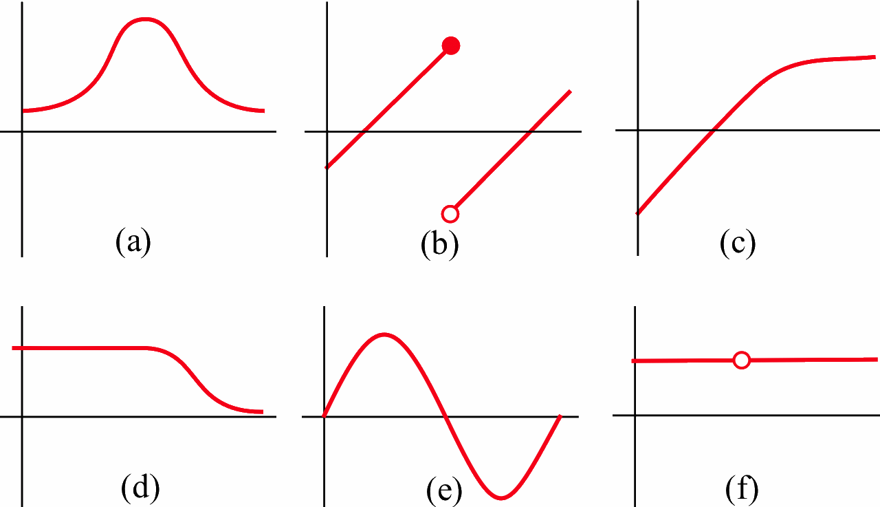
2. The figure below shows six graphs, three of which are derivatives of the other three. Match the functions with their derivatives.
   

In Problems 3–6, find the slope \(m_{\mbox{sec}}\) of the secant line through the two given points and then calculate \(\displaystyle m_{\mbox{tan}} = \lim_{h\to 0} \, m_{\mbox{sec}}\).

3. \(f(x) = x^2\)
   1. \((-2,4)\), \((-2+h, (-2+h)^2)\)
   2. \((0.5, 0.25)\), \((0.5+h, (0.5+h)^2)\)
4. \(f(x) = 3 + x^2\)
   1. \((1,4)\), \((1+h, 3+(1+h)^2)\)
   2. \((x, 3 + x^2)\), \((x+h , 3 + (x+h)^2)\)
5. \(f(x) = 7x - x^2\)
   1. \((1, 6)\), \((1+h, 7(1+h) - (1+h)^2)\)
   2. \((x, 7x - x^2)\), \((x+h, 7(x+h) - (x+h)^2)\)
6. \(f(x) = x^3 + 4x\)
   1. \((1, 5)\), \((1+h, (1+h)^3 + 4(1+h))\)
   2. \((x, x^3 + 4x)\), \((x+h, (x+h)^3 + 4(x+h))\)
7. Use the graph below to estimate the values of these limits.
   
   (It helps to recognize what the limit represents.)
   1. \(\displaystyle \lim_{h\to 0} \, \frac{f(0+ h) - f(0)}{h}\)
   2. \(\displaystyle \lim_{h\to 0} \, \frac{f(1+ h) - f(1)}{h}\)
   3. \(\displaystyle \lim_{w\to 0} \, \frac{f(2+ w) - 1}{w}\)
   4. \(\displaystyle \lim_{h\to 0} \, \frac{f(3+ h) - f(3)}{h}\)
   5. \(\displaystyle \lim_{h\to 0} \, \frac{f(4+ h) - f(4)}{h}\)
   6. \(\displaystyle \lim_{s\to 0} \, \frac{f(5+ s) - f(5)}{s}\)
8. Use the graph below to estimate the values of these limits.
   
   1. \(\displaystyle \lim_{h\to 0} \, \frac{g(0+ h) - g(0)}{h}\)
   2. \(\displaystyle \lim_{h\to 0} \, \frac{g(1+ h) - g(1)}{h}\)
   3. \(\displaystyle \lim_{w\to 0} \, \frac{g(2+ w) - 2}{w}\)
   4. \(\displaystyle \lim_{h\to 0} \, \frac{g(3+ h) - g(3)}{h}\)
   5. \(\displaystyle \lim_{h\to 0} \, \frac{g(4+ h) - g(4)}{h}\)
   6. \(\displaystyle \lim_{s\to 0} \, \frac{g(5+ s) - g(5)}{s}\)

In Problems 9–12, use the definition of the derivative to calculate \(f'(x)\) and then evaluate \(f'(3)\).

9. \(f(x) = x^2 + 8\)
10. \(f(x) = 5x^2 - 2x\)
11. \(f(x) = 2x^3 -5x\)
12. \(f(x) = 7x^3 + x\)
13. Graph \(f(x) = x^2\), \(g(x) = x^2 + 3\) and \(h(x) = x^2- 5\). Calculate the derivatives of \(f\), \(g\) and \(h\).
14. Graph \(f(x) = 5x\), \(g(x) = 5x + 2\) and \(h(x) = 5x - 7\). Calculate the derivatives of \(f\), \(g\) and \(h\).

In Problems 15–18, find the slopes and equations of the lines tangent to \(y = f(x)\) at the given points.

15. \(f(x) = x^2 + 8\) at \((1,9)\) and \((-2,12)\).
16. \(f(x) = 5x^2- 2x\) at \((2, 16)\) and \((0,0)\).
17. \(f(x) = \sin(x)\) at \((\pi, 0)\) and \((\frac{\pi}{2},1)\).
18. \(f(x) = \left| x + 3 \right|\) at \((0,3)\) and \((-3,0)\).
19. 1. Find an equation of the line tangent to the graph of \(y = x^2 + 1\) at the point \((2,5)\).
    2. Find an equation of the line perpendicular to the graph of \(y = x^2 + 1\) at \((2,5)\).
    3. Where is the line tangent to the graph of \(y = x^2 + 1\) horizontal?
    4. Find an equation of the line tangent to the graph of \(y = x^2 + 1\) at the point \((p,q)\).
    5. Find the point(s) \((p,q)\) on the graph of \(y = x^2 + 1\) so the tangent line to the curve at \((p,q)\) goes through the point \((1, -7)\).
20. 1. Find an equation of the line tangent to the graph of \(y = x^3\) at the point \((2,8)\).
    2. Where, if ever, is the line tangent to the graph of \(y = x^3\) horizontal?
    3. Find an equation of the line tangent to the graph of \(y = x^3\) at the point \((p,q)\).
    4. Find the point(s) \((p,q)\) on the graph of \(y = x^3\) so the tangent line to the curve at \((p,q)\) goes through the point \((16,0)\).
21. 1. Find the angle that the line tangent to \(y = x^2\) at \((1,1)\) makes with the \(x\)-axis.
    2. Find the angle that the line tangent to \(y = x^3\) at \((1,1)\) makes with the \(x\)-axis.
    3. The curves \(y = x^2\) and \(y = x^3\) intersect at the point \((1,1)\). Find the angle of intersection of the two curves (actually the angle between their tangent lines) at the point \((1,1)\).
22. The figure below shows the graph of \(y = f(x)\). Sketch a graph of \(y = f'(x)\).
    
23. The figure below shows the graph of the height of an object at time \(t\).
    
    Sketch a graph of the object’s upward velocity. What are the units for each axis on the velocity graph?
24. Fill in the table with units for \(f'(x)\).

    units for x	units for f(x)	units for f'(x)
    hours	miles
    people	automobiles
    dollars	pancakes
    days	trout
    seconds	miles per second
    seconds	gallons
    study hours	test points

25. A rock dropped into a deep hole will drop \(d(x) = 16x^2\) feet in \(x\) seconds.
    1. How far into the hole will the rock be after \(4\) seconds? After \(5\) seconds?
    2. How fast will it be falling at exactly \(4\) seconds? After \(5\) seconds? After \(x\) seconds?
26. It takes \(T(x) = x^2\) hours to weave \(x\) small rugs. What is the marginal production time to weave a rug? (Be sure to include the units with your answer.)
27. It costs \(C(x) = \sqrt{x}\) dollars to produce \(x\) golf balls. What is the marginal production cost to make a golf ball? What is the marginal production cost when \(x = 25\)? When \(x= 100\)? (Include units.)
28. Define \(A(x)\) to be the {\bf area} bounded by the \(t\)- and \(y\)-axes, the line \(y = 5\) and a vertical line at \(t = x\):
    
    1. Evaluate \(A(0)\), \(A(1)\), \(A(2)\) and \(A(3)\).
    2. Find a formula for \(A(x)\) valid for \(x \geq 0\).
    3. Determine \(A'(x)\).
    4. What does \(A'(x)\) represent?
29. Define \(A(x)\) to be the {\bf area} bounded by the \(t\)-axis, the line \(y = t\), and a vertical line at \(t =x\):
    
    1. Evaluate \(A(0)\), \(A(1)\), \(A(2)\) and \(A(3)\).
    2. Find a formula for \(A(x)\) valid for \(x \geq 0\).
    3. Determine \(A'(x)\).
    4. What does \(A'(x)\) represent?
30. Compute each derivative.
    1. \(\mbox{D}( x^{12} )\)
    2. \(\displaystyle \frac{d}{dx} (\sqrt[7]{x})\)
    3. \(\displaystyle \mbox{D}\left(\frac{1}{x^3} \right)\)
    4. \(\displaystyle \frac{d}{dx}( x^c)\)
    5. \(\mbox{D}( \left| x-2 \right| )\)
31. Compute each derivative.
    1. \(\mbox{D}( x^{9} )\)
    2. \(\displaystyle \frac{d}{dx} (x^{\frac23} )\)
    3. \(\displaystyle \mbox{D}\left(\frac{1}{x^4} \right)\)
    4. \(\displaystyle \frac{d}{dx}( x^{\pi})\)
    5. \(\mbox{D}( \left| x+5 \right| )\)

In Problems 32–37, find a function \(f\) that has the given derivative. (Each problem has several correct answers, just find one of them.)

32. \(f'(x) = 4x + 3\)
33. \(f'(x) = 3x^2 + 8x\)
34. \(\mbox{D}( f(x) ) = 12x^2 - 7\)
35. \(f'(t) = 5\cos(t)\)
36. \(\frac{d}{dx} f(x) = 2x - \sin(x)\)
37. \(\mbox{D}( f(x) ) = x + x^2\)