2.3: More Differentiation Patterns

Polynomials are very useful, but they are not the only functions we need. This section uses the ideas of the two previous sections to develop techniques for differentiating powers of functions, and to determine the  derivatives of some particular functions that occur often in applications: the trigonometric and exponential functions.

As you focus on learning how to differentiate different types and combinations of functions, it is important to remember what derivatives are and what they measure. Calculators and computers are  available to calculate derivatives. Part of your job as a professional will be to decide which functions need to be differentiated and how to use the resulting derivatives. You can succeed at that only if you  understand what a derivative is and what it measures.

A Power Rule for Functions: \(\mbox{D}( f^n(x) )\)

If we apply the Product Rule to the product of a function with itself, a pattern emerges.

\begin{align*}
 & \mbox{D}( f^2 ) & &= & \mbox{D}( f\cdot f ) & &=\ & &f\cdot \mbox{D}( f ) & &+\ \ &f\cdot \mbox{D}( f ) &  &= &      &     & &     &  &                     &= & &2f\cdot\mbox{D}(f) &\\
& \mbox{D}( f^3 ) & &= & \mbox{D}( f^2\cdot f ) & &=\ & &f^2\cdot \mbox{D}( f ) & &+\ \ &f\cdot \mbox{D}( f^2 ) & &= & &f^2\cdot \mbox{D}( f ) & &+ & &f\cdot 2f\cdot\mbox{D}(f)   &= & &3f^2\cdot\mbox{D}(f) &\\
& \mbox{D}( f^4 ) & &= & \mbox{D}( f^3\cdot f ) & &=\ & &f^3\cdot \mbox{D}( f ) & &+\ \ &f\cdot \mbox{D}( f^3 ) & &= & &f^3\cdot \mbox{D}( f ) & &+ & &f\cdot 3f^2\cdot\mbox{D}(f) &= & &4f^3\cdot\mbox{D}(f) &
\end{align*}

Practice \(\PageIndex{1}\)

What is the pattern here? What do you think the results will be for \(\mbox{D}( f^5 )\) and \(\mbox{D}( f^{13} )\)?

Answer

The pattern is \(\mbox{D}( f^n (x) ) = n \cdot f^{n-1}(x) \cdot \mbox{D}( f(x) )\): \(\mbox{D}(f^5(x)) = 5f^4(x)\cdot \mbox{D}(f(x))\) and \(\mbox{D}( f^{13}(x)) = 13 f^{12}(x)\cdot \mbox{D}(f(x))\)

We could keep differentiating higher and higher powers of \(f(x)\) by writing them as products of lower powers of \(f(x)\) and using the Product Rule, but the Power Rule for Functions guarantees that the pattern we just saw for the small integer powers also works for all constant powers of functions.

Power Rule for Functions

If: \(p\) is any constant

then: \(\mbox{D}( f^p(x) ) = p \cdot f^{p-1}(x)\cdot \mbox{D}( f(x) )\)

The Power Rule for Functions is a special case of a more general theorem, the Chain Rule, which we will examine in Section 2.4, so we will wait until then to prove the Power Rule for Functions.

Example \(\PageIndex{1}\)

Use the Power Rule for Functions to find:

1. \(\mbox{D}((x^3-5)^2)\)
2. \(\displaystyle \frac{d}{dx}\left(\sqrt{2x+3x^5}\right)\)
3. \(\mbox{D}(\sin^2(x))\) (Remember: \(\sin^2(x) = \left[\sin(x)\right]^2\))

Solution

1. To match the pattern of the Power Rule for \(\mbox{D}((x^3-5)^2)\), let \(f(x) = x^3- 5\) and \(p = 2\). Then: \begin{align*} \mbox{D}((x^3-5)^2) &= \mbox{D}( f^p(x) ) = p \cdot f^{p-1}(x)\cdot\mbox{D}( f(x) )\\ &= 2(x^3- 5)^1 \mbox{D}(x^3- 5) = 2(x^3- 5 )(3x^2) = 6x^2(x^3- 5)\end{align*}(Check that you get the same answer by first expanding \((x^3-5)^2\) and then taking the derivative.)
2. To match the pattern for \(\displaystyle \frac{d}{dx}\left(\sqrt{2x+3x^5}\right) = \frac{d}{dx}\left((2x+3x^5)^{\frac12}\right)\), let \(f(x) = 2x + 3x^5\) and take p = \(\frac12\). Then: \begin{align*} \frac{d}{dx}\left(\sqrt{2x+3x^5}\right) &= \frac{d}{dx}\left(f^p(x)\right) = p \cdot f^{p-1}(x)\cdot \frac{d}{dx}( f(x) )\\ &= \frac12 (2x + 3x^5)^{-\frac12}\frac{d}{dx}(2x + 3x^5)\\ &= \frac12 (2x + 3x^5)^{-\frac12}(2 + 15x^4) = \frac{2 + 15x^4}{2\sqrt{2x + 3x^5}} \end{align*}
3. To match the pattern for \(\mbox{D}(\sin^2(x))\), let \(f(x) = \sin(x)\) and \(p = 2\): \begin{align*} \mbox{D}(\sin^2(x) ) &= \mbox{D}( f^p(x) ) = p\cdot f^{p-1}(x)\cdot\mbox{D}( f(x) )\\ &= 2\sin^1(x) \mbox{D}( \sin(x) ) = 2\sin(x)\cos(x) \end{align*}(We could also rewrite this last expression as \(\sin(2x)\).)

Practice \(\PageIndex{2}\)

Use the Power Rule for Functions to find:

1. \(\displaystyle \frac{d}{dx}\left((2x^5-\pi)^2\right)\)
2. \(\displaystyle \mbox{D}\left(\sqrt{x+7x^2}\right)\)
3. \(\mbox{D}(\cos^4(x))\)

Answer

\(\displaystyle \frac{d}{dx} (2x^5- \pi)^2 = 2(2x^5-\pi)^1 \mbox{D}( 2x^5- \pi ) = 2(2x^5- \pi)(10x^4) = 40x^9 - 20\pi x^4\)

\(\displaystyle \mbox{D}\left( (x + 7x^2)^{\frac12}\right) = \frac12 (x + 7x^2)^{-\frac12} \mbox{D}( x + 7x^2) = \frac{1 + 14x}{2 \sqrt{x + 7x^2}}\)

\(\displaystyle \mbox{D}\left( (\cos(x) )^4\right) = 4( \cos(x) )^3 \mbox{D}( \cos(x) ) = 4( \cos(x) )^3( -\sin(x) ) = -4\cos^3(x) \sin(x)\)

Example \(\PageIndex{2}\)

Use calculus to show that the line tangent to the circle \(x^2 + y^2 = 25\) at the point \((3,4)\) has slope \(-\frac34\).

Solution

The top half of the circle is the graph of \(f(x) = \sqrt{25 - x^2}\) so:\[f'(x) = \mbox{D}\left( (25 - x^2)^{\frac12})\right) = \frac12  (25 - x^2)^{-\frac12} \cdot \mbox{D}(25 - x^2) = \frac{-x}{\sqrt{25 - x^2}}\nonumber\]and \(\displaystyle f'(3) = \frac{-3}{\sqrt{25 - 3^2}} = -\frac34\). As a check, you can verify that the slope of the radial line through the center of the circle \((0,0)\) and the point \((3,4)\) has slope \(\frac43\) and is perpendicular to the tangent line that has a slope of \(-\frac34\).

Derivatives of Trigonometric Functions

We have some general rules that apply to any elementary combination of differentiable functions, but in order to use the rules we still need to know the derivatives of some basic functions. Here we will begin to add to the list of functions whose derivatives we know.

We already know the derivatives of the sine and cosine functions, and each of the other four trigonometric functions is just a ratio involving sines or cosines. Using the Quotient Rule, we can easily differentiate the rest of  the trigonometric functions.

Theorem

• \(\mbox{D}(\tan(x)) = \sec^2(x)\)
• \(\mbox{D}(\sec(x)) = \sec(x) \cdot \tan(x)\)
• \(\mbox{D}(\cot(x)) = -\csc^2(x)\)
• \(\mbox{D}(\csc(x)) = -\csc(x) \cdot \cot(x)\)

Proof

From trigonometry, we know \(\displaystyle \tan(x) = \frac{\sin(x)}{\cos(x)}\), \(\displaystyle \cot(x) = \frac{\cos(x)}{\sin(x)}\), \(\displaystyle \sec(x) = \frac{1}{\cos(x)}\) and \(\displaystyle \csc(x) = \frac{1}{\sin(x)}\). 

From calculus, we already know \(\mbox{D}( \sin(x) ) = \cos(x)\) and \(\mbox{D}( \cos(x) ) = -\sin(x)\). So:
\begin{align*}
\mbox{D}( \tan(x) ) &= \mbox{D}\left(\frac{\sin(x)}{\cos(x)}\right) = \frac{\cos(x)\cdot\mbox{D}(\sin(x) ) - \sin(x)\cdot\mbox{D}( \cos(x) )}{( \cos(x) )^2}\\
&= \frac{\cos(x) \cdot \cos(x) - \sin(x)(-\sin(x))}{\cos^2(x)}\\
&= \frac{\cos^2(x) + \sin^2(x)}{\cos^2(x)} = \frac{1}{\cos^2(x)} = \sec^2(x)\end{align*}
Similarly:
\begin{align*}
\mbox{D}( \sec(x) ) &= \mbox{D}\left(\frac{1}{\cos(x)}\right) = \frac{\cos(x)\cdot\mbox{D}(1) - 1\cdot\mbox{D}( \cos(x) )}{( \cos(x) )^2}\\
&= \frac{\cos(x) \cdot 0 - (-\sin(x))}{\cos^2(x)}\\
&= \frac{\sin(x)}{\cos^2(x)} = \frac{1}{\cos(x)} \cdot \frac{\sin(x)}{\cos(x)} = \sec(x)\cdot\tan(x)\end{align*}
Instead of the Quotient Rule, we could have used the Power Rule to calculate \(\mbox{D}(\sec(x) ) = \mbox{D}( (\cos(x))^{-1})\).

Practice \(\PageIndex{3}\)

Use the Quotient Rule on \(\displaystyle f(x) = \cot(x) =  \frac{\cos(x)}{\sin(x)}\) to prove that \(f'(x) = -\csc^2(x)\).

Answer

Mimicking the proof for the derivative of \(\tan(x)\):
\begin{align*}\mbox{D}\left(\frac{\cos(x)}{\sin(x)}\right) &= \frac{\sin(x)\cdot \mbox{D}(\cos(x) ) - \cos(x)\cdot \mbox{D}( \sin(x))}{(\sin(x))^2}\\
&= \frac{\sin(x)(-\sin(x) ) - \cos(x)(\cos(x) )}{\sin^2(x)}\\ &= \frac{-(\sin^2(x) + \cos^2(x))}{\sin^2(x)} = \frac{-1}{\sin^2(x)} = -\csc^2(x)\end{align*}

Practice \(\PageIndex{4}\)

Prove that \(\mbox{D}(\csc(x) ) = -\csc(x)\cdot\cot(x)\). The justification of this result is very similar to the justification for \(\mbox{D}(\sec(x))\).

Answer

Mimicking the proof for the derivative of \(\sec(x)\):
\begin{align*}
\mbox{D}(\csc(x) ) &= \mbox{D}\left(\frac{1}{\sin(x)}\right) = \frac{\sin(x)\cdot\mbox{D}( 1 ) - 1\cdot\mbox{D}(\sin(x)}{\sin^2(x)}\\
&= \frac{\sin(x)\cdot 0 - \cos(x)}{\sin^2(x)} = -\frac{1}{\sin(x)} \cdot \frac{\cos(x)}{\sin(x)} = -\cot(x)\csc(x)\end{align*}

Practice \(\PageIndex{5}\)

Find:

1. \(\mbox{D}( x^5\tan(x))\)
2. \(\displaystyle \frac{d}{dt}\left(\frac{\sec(t)}{t}\right)\)
3. \(\mbox{D}\left(\sqrt{\cot(x)-x}\right)\)

Answer

\(\mbox{D}(x^5\cdot \tan(x) ) = x^5 \mbox{D}( \tan(x) ) + \tan(x) \mbox{D}( x^5) = x^5\sec^2(x) + \tan(x) (5x^4)\)

\(\displaystyle \frac{d}{dt} \left(\frac{\sec(t)}{t}\right) = \frac{t\mbox{D}( \sec(t) ) - \sec(t)\mbox{D}( t )}{t^2} = \frac{t\sec(t)\tan(t) - \sec(t)}{t^2}\)

\begin{align*}\mbox{D}\left( (\cot(x) - x )^{\frac12} \right) &= \frac12 (\cot(x) - x )^{-\frac12} \mbox{D}( \cot(x) - x )\\
&= \frac12 (\cot(x) - x )^{-\frac12}(-\csc^2(x) - 1) = \frac{-\csc^2(x) - 1}{2\sqrt{\cot(x) - x}}\end{align*}

Derivatives of Exponential Functions

We can estimate the value of a derivative of an exponential function (a function of the form \(f(x) = a^x\) where \(a>0\)) by estimating the slope of the line tangent to the graph of such a function, or we can numerically approximate those slopes.

Example \(\PageIndex{3}\)

Estimate the value of the derivative of \(f(x) = 2^x\) at the point \((0, 2^0) = ( 0, 1 )\) by approximating the slope of the line tangent to \(f(x) = 2^x\) at that point.

Solution

We can get estimates from the graph of \(f(x) = 2^x\) by carefully graphing \(y = 2^x\) for small values of \(x\) (so that \(x\) is near \(0\)), sketching secant lines, and then measuring the slopes of the secant lines:

We can also estimate the slope numerically by using the definition of the derivative:\[f'(0) = \lim_{h\to 0} \, \frac{f(0+ h) - f(0)}{h} = \lim_{h\to 0} \, \frac{2^{0+h}-2^0}{h} = \lim_{h\to 0} \, \frac{2^h - 1}{h}\nonumber\]and evaluating \(\displaystyle \frac{2^h - 1}{h}\) for some very small values of \(h\). From the table below we can see that \(f'(0) \approx 0.693\).

\(h\)	\(\frac{2^h-1}{h}\)	\(\frac{3^h-1}{h}\)	\(\frac{e^h-1}{h}\)
\(+0.1\)	\(0.717734625\)
\(-0.1\)	\(0.669670084\)
\(+0.01\)	\(0.695555006\)
\(-0.01\)	\(0.690750451\)
\(+0.001\)	\(0.693387463\)
\(-0.001\)	\(0.692907009\)
\(\downarrow\)	\(\downarrow\)	\(\downarrow\)	\(\downarrow\)
\(0\)	\(\approx0.693\)	\(\approx 1.099\)	\(1\)

Practice \(\PageIndex{6}\)

Fill in the table above for \(\displaystyle \frac{3^h - 1}{h}\) and show that the slope of the line tangent to \(g(x) = 3^x\) at \((0,1)\) is approximately \(1.099\).

Answer

Filling in values for both \(3^x\) and \(e^x\):

\(h\)	\(\frac{2^h-1}{h}\)	\(\frac{3^h-1}{h}\)	\(\frac{e^h-1}{h}\)
\(+0.1\)	\(0.717734625\)	\(1.161231740\)	\(1.0517091808\)
\(-0.1\)	\(0.669670084\)	\(1.040415402\)	\(0.9516258196\)
\(+0.01\)	\(0.695555006\)	\(1.104669194\)	\(1.0050167084\)
\(-0.01\)	\(0.690750451\)	\(1.092599583\)	\(0.9950166251\)
\(+0.001\)	\(0.693387463\)	\(1.099215984\)	\(1.0005001667\)
\(-0.001\)	\(0.692907009\)	\(1.098009035\)	\(0.9995001666\)
\(\downarrow\)	\(\downarrow\)	\(\downarrow\)	\(\downarrow\)
\(0\)	\(\approx0.693\)	\(\approx 1.0986\)	\(1\)

At \((0,1)\), the slope of the tangent to \(y = 2^x\) is less than \(1\) and the slope of the tangent to \(y = 3^x\) is slightly greater than \(1\). You might expect that there is a number \(b\) between \(2\) and \(3\) so that the slope of the tangent to \(y = b^x\) is exactly \(1\). Indeed, there is such a number, \(e \approx 2.71828182845904\), with\[\lim_{h\to 0} \, \frac{e^h - 1}{h} =1\nonumber\]The number \(e\) is irrational and plays a very important role in calculus and applications. (In fact, \(e\) is a “transcendental” number, which means that it is not the root of any polynomial equation with rational coefficients.)

We have not proved that this number \(e\) with the desired limit property actually exists, but if we assume it does, then it becomes relatively straightforward to calculate \(\mbox{D}(e^x)\). (Don't worry — we’ll tie up some of these loose ends in Chapter 7.)

Theorem

\(\mbox{D}( e^x) = e^x\) 

Proof

Using the definition of the derivative:
\begin{align*}
\mbox{D}(e^x) &= \lim_{h\to 0} \, \frac{e^{x+h} - e^x}{h} = \lim_{h\to 0} \, \frac{e^x\cdot e^h - e^x}{h}\\
&= \lim_{h\to 0} \, e^x \cdot \frac{e^h - 1}{h} = \lim_{h\to 0} \, e^x \cdot \lim_{h\to 0} \, \frac{e^h - 1}{h}\\
&= e^x \cdot 1 = e^x\end{align*}
The function \(f(x) = e^x\) is its own derivative: \(f'(x) = f(x)\).

Graphically: the height of \(f(x) = e^x\) at any point and the slope of the tangent to \(f(x) = e^x\) at that point are the same: as the graph gets higher, its slope gets steeper. (Notice that the limit property of \(e\) that we assumed was true actually says that for \(f(x) = e^x\), \(f'(0)=1\). So knowing the derivative of \(f(x) = e^x\) at a single point (\(x=0\)) allows us to determine its derivative at every other point.)

Example \(\PageIndex{4}\)

Find:

1. \(\displaystyle \frac{d}{dt}\left(t\cdot e^t\right)\)
2. \(\displaystyle \mbox{D}\left( \frac{e^x}{\sin(x)} \right)\)
3. \(\mbox{D}( e^{5x})\)

Solution

1. Using the Product Rule with \(f(t) = t\) and \(g(t) = e^t\):\[\frac{d}{dt} \left(t\cdot e^t\right) = t\cdot \mbox{D}(e^t) + e^t \cdot \mbox{D}(t) = t\cdot e^t + e^t \cdot 1 = (t+1)e^t\nonumber\]
2. Using the Quotient Rule with \(f(x) = e^x\) and \(g(x) = \sin(x)\): \begin{align*} \mbox{D}\left( \frac{e^x}{\sin(x)} \right) &= \frac{\sin(x)\cdot \mbox{D}(e^x) - e^x\cdot \mbox{D}(\sin(x))}{\left[\sin(x)\right]^2}\\ &= \frac{\sin(x)\cdot e^x - e^x(\cos(x))}{\sin^2(x)} \end{align*}
3. Using the Power Rule for Functions with \(f(x) = e^x\) and \(p = 5\): \[\mbox{D}((e^x)^5) = 5(e^x)^4\cdot \mbox{D}( e^x) = 5e^{4x} \cdot e^x = 5e^{5x}\nonumber\]where we have rewritten \(e^{5x}\) as \((e^x)^5\).

Practice \(\PageIndex{7}\)

Find:

1. \(\mbox{D}( x^3 e^x)\)
2. \(\mbox{D}( ( e^x )^3)\).

Answer

\(\mbox{D}( x^3 e^x) = x^3\mbox{D}(e^x) + e^x\mbox{D}(x^3) = x^3 e^x +e^x\cdot 3x^2 = x^2e^x(x + 3)\)

\(\displaystyle \mbox{D}\left( ( e^x )^3\right) = 3\left( e^x \right)^2 \mbox{D}( e^x) = 3e^{2x} \cdot e^x = 3 e^{3x}\)

Higher Derivatives: Derivatives of Derivatives

The derivative of a function \(f\) is a new function \(f'\) and if this new function is differentiable we can calculate the derivative of this new function to get the derivative of the derivative of \(f\), denoted by \(f''\) and called the {\bf second derivative} of \(f\). 

For example, if \(f(x) = x^5\) then \(f'(x) = 5x^4\) and \(f''(x) = (f'(x))' = (5x^4)' = 20x^3\).

Definitions

Given a differentiable function \(f\):

• the first derivative is \(f'(x)\), the rate of change of \(f\).
• the second derivative is \(f''(x) = (f'(x))'\), the rate of change of \(f'\).
• the third derivative is \(f'''(x) = (f''(x))'\), the rate of change of \(f''\).

For \(y = f(x)\), we write \(\displaystyle f'(x) = \frac{dy}{dx}\), so we can extend that notation to write \(\displaystyle f''(x) = \frac{d}{dx}\left(\frac{dy}{dx}\right) = \frac{d^2 y}{dx^2}\), \(\displaystyle f'''(x) = \frac{d}{dx}\left(\frac{d^2y}{dx^2}\right) = \frac{d^3 y}{dx^3}\) and so on.

Practice \(\PageIndex{8}\)

Find \(f'\), \(f''\) and \(f'''\) for \(f(x) = 3x^7\), \(f(x) = \sin(x)\) and \(f(x) = x\cdot\cos(x)\).

Answer

\(f(x) = 3x^7 \Rightarrow f'(x) = 21x^6\Rightarrow f''(x) = 126x^5 \Rightarrow f'''(x) = 630x^4\)

\(f(x) = \sin(x) \Rightarrow f'(x) = \cos(x) \Rightarrow f''(x) = -\sin(x) \Rightarrow f'''(x) = -\cos(x)\)

\(f(x) = x\cdot \cos(x) \Rightarrow f'(x) = -x\sin(x) + \cos(x) \Rightarrow f''(x) = -x \cos(x) - 2\sin(x) \Rightarrow f'''(x) = x\sin(x) - 3\cos(x)\)

If \(f(x)\) represents the position of a particle at time \(x\), then \(v(x) = f'(x)\) will represent the velocity (rate of change of the position) of the particle and \(a(x) = v'(x) = f''(x)\) will represent the acceleration (the rate of change of the velocity) of the particle.

Example \(\PageIndex{5}\)

The height (in feet) of a particle at time \(t\) seconds is given by \(t^3 - 4t^2 + 8t\). Find the height, velocity and acceleration of the particle when \(t = 0\), \(1\) and \(2\) seconds.

Solution

\(f(t) = t^3- 4t^2 + 8t\) so \(f(0) = 0\) feet, \(f(1) = 5\) feet and \(f(2) = 8\) feet. The velocity is given by \(v(t) = f'(t) = 3t^2- 8t + 8\) so \(v(0) = 8\) ft/sec, \(v(1) = 3\) ft/sec and \(v(2) = 4\) ft/sec. At each of these times the velocity is positive and the particle is moving upward (increasing in height). The acceleration is \(a(t) = 6t - 8\) so \(a(0) = -8\) ft/sec\)^2\), \(a(1) = -2\) ft/sec\)^2\) and \(a(2) = 4\) ft/sec\)^2\).

We will examine the geometric (graphical) meaning of the second derivative in the next chapter.

A Really “Bent” Function

In Section 1.2 we saw that the “holey” function\[h(x) = \left\{
\begin{array}{rl}
{ 2 } & { \text{if } x \text{ is a rational number} } \\
{ 1 } & { \text{if } x \text{ is an irrational number} } \end{array}\right.\nonumber\]is discontinuous at every value of \(x\), so \(h(x)\) is not differentiable anywhere. We can create graphs of  continuous functions that are not differentiable at several places just by putting corners at those places, but how many corners can a continuous function have? How badly can a continuous function fail to be differentiable?

In the mid-1800s, the German mathematician Karl Weierstrass surprised and even shocked the mathematical world by creating a function that was {\bf continuous everywhere but differentiable nowhere} — a function whose graph was everywhere connected and everywhere bent! He used techniques we have not investigated yet, but we can begin to see how such a function could be built.

Start with a function \(f_1\) that zigzags between the values \(\frac12\) and \(-\frac12\) and has a “corner” at each integer:

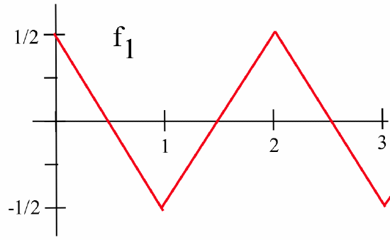
This starting function \(f_1\) is continuous everywhere and is differentiable everywhere except at the integers. Next create a list of functions \(f_2\), \(f_3\), \(f_4\), … , each of which is “shorter” than the previous one but with many more “corners” than the previous one. For example, we might make \(f_2\) zigzag between the values \(\frac14\) and \(-\frac14\) and have “corners” at \(\pm\frac12\), \(\pm\frac32\), \(\pm\frac52\), etc.:

\(f_3\) zigzag between \(\frac19\) and \(-\frac19\) and have “corners” at \(\pm\frac13\), \(\pm\frac23\), \(\pm\frac33 = \pm1\), etc.:

and so on. If we add \(f_1\) and \(f_2\), we get a continuous function (because the sum of two continuous functions is continuous) with corners at \(0\), \(\pm\frac12\), \(\pm 1\), \(\pm \frac32\), … . If we then add \(f_3\) to the previous sum, we get a new continuous function with even more corners. If we continue adding the functions in our list “indefinitely,” the final result will be a continuous function that is differentiable nowhere.

We haven’t developed enough mathematics here to precisely describe what it means to add an infinite number of functions together or to verify that the resulting function is nowhere differentiable — but we will. You can at least start to imagine what a strange, totally “bent” function it must be. Until Weierstrass created his “everywhere continuous, nowhere differentiable” function, most mathematicians thought a continuous function could only be “bad” in a few places. Weierstrass’ function was (and is) considered “pathological,” a great example of how bad something can be. The mathematician Charles Hermite expressed a reaction shared by many when they first encounter the Weierstrass function: “I turn away with fright and horror from this lamentable evil of functions which do not have derivatives.”

Important Results

Power Rule for Functions: \(\mbox{D}(f^p(x)) = p\cdot f^{p-1}(x)\cdot\mbox{D}( f(x) )\)

Derivatives of the Trigonometric Functions:

\(\mbox{D}( \sin(x) ) = \cos(x)\), \(\mbox{D}( \cos(x) ) = -\sin(x)\)

\(\mbox{D}( \tan(x) ) = \sec^2(x)\), \(\mbox{D}( \cot(x) ) = -\csc^2(x)\)

\(\mbox{D}( \sec(x) ) = \sec(x) \tan(x)\), \(\mbox{D}( \csc(x) ) = -\csc(x)\cot(x)\)

Derivative of the Exponential Function: \(\mbox{D}(e^x) = e^x\)

Problems

1. Let \(f(1) = 2\) and \(f'(1) = 3\). Find the values of each of the following derivatives at \(x = 1\).
   1. \(\mbox{D}(f^2(x))\)
   2. \(\mbox{D}(f^5(x))\)
   3. \(\mbox{D}(\sqrt{f(x)})\)
2. Let \(f(2) = -2\) and \(f'(2) = 5\). Find the values of each of the following derivatives at \(x = 2\).
   1. \(\mbox{D}(f^2(x))\)
   2. \(\mbox{D}(f^{-3}(x))\)
   3. \(\mbox{D}(\sqrt{f(x)})\)
3. For \(x=1\) and \(x=3\) estimate the values of \(f(x)\), whose graph appears below:
   
   as well as \(f'(x)\) and
   1. \(\displaystyle \frac{d}{dx}\left(f^2(x)\right)\)
   2. \(\mbox{D}\left(f^3(x)\right)\)
   3. \(\mbox{D}\left(f^5(x)\right)\)
4. For \(x=0\) and \(x=2\) estimate the values of \(f(x)\) (from the previous Problem), \(f'(x)\) and
   1. \(\mbox{D}\left(f^2(x)\right)\)
   2. \(\displaystyle \frac{d}{dx}\left(f^3(x)\right)\)
   3. \(\displaystyle \frac{d}{dx}\left(f^5(x)\right)\)

In Problems 5–10, find \(f'(x)\).

10. \(f(x) = (2x - 8)^5\)
11. \(f(x) = (6x - x^2)^{10}\)
12. \(f(x) = x\cdot (3x + 7)^5\)
13. \(f(x) = (2x + 3)^6 \cdot (x - 2)^4\)
14. \(f(x) = \sqrt{x^2 + 6x - 1}\)
15. \(\displaystyle f(x) = \frac{x - 5}{(x + 3)^4}\)
16. A mass attached to the end of a spring is at a height of \(h(t) = 3 - 2\sin(t)\) feet above the floor \(t\) seconds after it is released.
    1. Graph \(h(t)\).
    2. At what height is the mass when it is released?
    3. How high does above the floor and how close to the floor does the mass ever get?
    4. Determine the height, velocity and acceleration at time \(t\). (Be sure to include the correct units.)
    5. Why is this an unrealistic model of the motion of a mass attached to a real spring?
17. A mass attached to a spring is at a height of \(\displaystyle h(t) = 3 - \frac{2\sin(t)}{1 + 0.1t^2}\) feet above the floor \(t\) seconds after it is released.
    1. Graph \(h(t)\).
    2. At what height is the mass when it is released?
    3. Determine the velocity of the mass at time \(t\).
    4. What happens to the height and the velocity of the mass a “long time” after it is released?
18. The kinetic energy \(K\) of an object of mass \(m\) and velocity \(v\) is \(\frac12 mv^2\).
    1. Find the kinetic energy of an object with mass \(m\) and height \(h(t) = 5t\) feet at \(t = 1\) and \(t = 2\) seconds.
    2. Find the kinetic energy of an object with mass \(m\) and height \(h(t) = t^2\) feet at \(t = 1\) and \(t = 2\) seconds.
19. An object of mass \(m\) is attached to a spring and has height \(h(t) = 3 + \sin(t)\) feet at time \(t\) seconds.
    1. Find the height and kinetic energy of the object when \(t = 1\), \(2\) and \(3\) seconds.
    2. Find the rate of change in the kinetic energy of the object when \(t = 1\), \(2\) and \(3\) seconds.
    3. Can \(K\) ever be negative? Can \(\displaystyle \frac{dK}{dt}\) ever be negative? Why?

In Problems 15–20, compute \(f'(x)\).

15. \(f(x) = x\cdot \sin(x)\)
16. \(f(x) = \sin^5(x)\)
17. \(f(x) = e^x- \sec(x)\)
18. \(f(x) = \sqrt{\cos(x) + 1}\)
19. \(f(x) = e^{-x} + \sin(x)\)
20. \(f(x) = \sqrt{x^2- 4x + 3}\)

In Problems 21–26, find an equation for the line tangent to the graph of \(y=f(x)\) at the given point.

21. \(f(x) = (x - 5)^7\) at \((4, -1)\)
22. \(f(x) = e^x\) at \((0,1)\)
23. \(f(x) = \sqrt{25 - x^2}\) at \((3,4)\)
24. \(f(x) = \sin^3(x)\) at \((\pi,0)\)
25. \(f(x) = (x - a)^5\) at \((a,0)\)
26. \(f(x) = x\cdot \cos^5(x)\) at \((0, 0)\)
27. 1. Find an equation for the line tangent to \(f(x) = e^x\) at the point \((3, e^3)\).
    2. Where will this tangent line intersect the \(x\)-axis?
    3. Where will the tangent line to \(f(x) = e^x\) at the point \((p, e^p)\) intersect the \(x\)-axis?

In Problems 28–33, calculate \(f'\) and \(f''\).

28. \(f(x) = 7x^2 + 5x - 3\)
29. \(f(x) = \cos(x)\)
30. \(f(x) = \sin( x )\)
31. \(f(x) = x^2\cdot \sin( x )\)
32. \(f(x) = x\cdot \sin(x)\)
33. \(f(x) = e^x \cdot \cos(x)\)
34. Calculate the first 8 derivatives of \(f(x) = \sin(x)\). What is the pattern? What is the 208th derivative of \(\sin(x)\)?
35. What will the second derivative of a quadratic polynomial be? The third derivative? The fourth derivative?
36. What will the third derivative of a cubic polynomial be? The fourth derivative?
37. What can you say about the \(n\)-th and \((n+1)\)-st derivatives of a polynomial of degree \(n\)?

In Problems 38–42, you are given \(f'\). Find a function \(f\) with the given derivative.

38. \(f'(x) = 4x + 2\)
39. \(f'(x) = 5e^x\)
40. \(f'(x) = 3\cdot \sin^2(x) \cdot \cos(x)\)
41. \(f'(x) = 5(1 + e^x)^4 \cdot e^x\)
42. \(f'(x) = e^x + \sin(x)\)
43. The function \(f(x)\) defined as\(f(x) = \left\{ \begin{array}{rl} { x\cdot\sin(\frac{1}{x}) } & { \text{if } x \neq 0 } \\ { 0 } & { \text{if } x = 0 } \end{array}\right.\) shown below is continuous at \(0\) because we can show (using the Squeezing Theorem) that \(\displaystyle \lim_{h\to 0} f(x) = 0 = f(0)\).
    
    Is \(f\) differentiable at \(0\)? To answer this question, use the definition of \(f'(0)\) and consider \[\lim_{h\to 0}\, \frac{f(0+ h) - f(0)}{h}\nonumber\]
44. The function \(f(x)\) defined as \(f(x) = \left\{ \begin{array}{rl} { x^2\cdot\sin(\frac{1}{x}) } & { \text{if } x \neq 0 } \\ { 0 } & { \text{if } x = 0 } \end{array}\right.\) shown below is continuous at \(0\) because we can show (using the Squeezing Theorem) that \(\lim_{h\to 0} f(x) = 0 = f(0)\).
    
    Is \(f\) differentiable at \(0\)? To answer this question, use the definition of \(f'(0)\) and consider \[\lim_{h\to 0}\, \frac{f(0+ h) - f(0)}{h}\nonumber\]

The number \(e\) appears in a variety of unusual situations. Problems 45–48 illustrate a few of these.

45. Use your calculator to examine the values of \(\displaystyle f(x) = \left( 1 + \frac{1}{x}\right)^x\) when \(x\) is relatively large (for example, \(x = 100\), \(1000\) and \(10,000\). Try some other large values for \(x\). If \(x\) is large, the value of \(f(x)\) is close to what number?
46. If you put \\)1 into a bank account that pays 1\% interest per year and compounds the interest \(x\) times a year, then after one year you will have \(\left(1 + \frac{0.01}{x}\right)^x\) dollars in the account.
    1. How much money will you have after one year if the bank calculates the interest once a year?
    2. How much money will you have after one year if the bank calculates the interest twice a year?
    3. How much money will you have after one year if the bank calculates the interest 365 times a year?
    4. How does your answer to part (c) compare with \(e^{0.01}\)?
47. Define \(n!\) to be the product of all positive integers from \(1\) through \(n\). For example, \(2! = 1\cdot 2 = 2\), \(3! = 1\cdot 2 \cdot 3 = 6\) and \(4! = 1\cdot 2 \cdot 3 \cdot 4 = 24\).
    1. Calculate the value of the sums: \begin{align*} s_1 &= 1 + \frac{1}{1!}\\ s_2 &= 1 + \frac{1}{1!} + \frac{1}{2!}\\ s_3 &= 1 + \frac{1}{1!} + \frac{1}{2!} + \frac{1}{3!}\\ s_4 &= 1 + \frac{1}{1!} + \frac{1}{2!} + \frac{1}{3!} + \frac{1}{4!}\\ s_5 &= 1 + \frac{1}{1!} + \frac{1}{2!} + \frac{1}{3!} + \frac{1}{4!} + \frac{1}{5!}\\ s_6 &= 1 + \frac{1}{1!} + \frac{1}{2!} + \frac{1}{3!} + \frac{1}{4!} + \frac{1}{5!} + \frac{1}{6!}\end{align*}
    2. What value do the sums in part (a) seem to be approaching?
    3. Calculate \(s_7\) and \(s_8\).
48. If it is late at night and you are tired of studying calculus, try the following experiment with a friend. Take the 2 through 10 of hearts from a regular deck of cards and shuffle these nine cards well. Have your friend do the same with the 2 through 10 of spades. Now compare your cards one at a time. If there is a match, for example you both play a 5, then the game is over and you win. If you make it through the entire nine cards with no match, then your friend wins. If you play the game {\bf many times}, then the ratio:\[\frac{\mbox{total number of games played}}{\mbox{number of times your friend wins}}\nonumber\]will be approximately equal to \(e\).