2.7: Newton’s Method

Newton’s method is a process that can find roots of functions whose graphs cross or just “kiss” the \(x\)-axis. Although this method is a bit harder to apply than the Bisection Algorithm, it often finds roots that the Bisection Algorithm misses, and it usually finds them faster.

Off on a Tangent

The basic idea of Newton’s Method is remarkably simple and graphical: at a point \((x, f(x))\) on the graph of \(f\), the tangent line to the graph “points toward” a root of \(f\), a place where the graph touches the \(x\)-axis.

To find a root of \(f\), we just pick a starting value \(x_0\), go to the point \((x_0 ,f(x_0))\) on the graph of \(f\), build a tangent line there, and follow the tangent line to where it crosses the \(x\)-axis, say at \(x_1\).

If \(x_1\) is a root of \(f\), we are done. If \(x_1\) is not a root of \(f\), then \(x_1\) is usually closer to the root than \(x_0\) was, and we can repeat the process, using \(x_1\) as our new starting point. Newton’s method is an iterative procedure — that is, the output from one application of the method becomes the starting point for the next application.

Let’s begin with the function \(f(x) = x^2- 5\), whose roots we already know (\(x = \pm\sqrt{5} \approx \pm 2.236067977\)), to illustrate Newton’s method.

First, pick some value for \(x_0\), say \(x_0 = 4\), and move to the point \((x_0 , f(x_0) ) = ( 4 , 11 )\) on the graph of \(f\). The tangent line to the graph of \(f\) at \((4, 11)\) “points to” a location on the \(x\)-axis that is closer to the root of \(f\) than the point we started with. We calculate this location on the \(x\)-axis by finding an equation of the line tangent to the graph of \(f\) at \((4, 11)\) and then finding where this line intersects the \(x\)-axis.

At \((4, 11)\), the line tangent to \(f\) has slope \(f'(4) = 2(4) = 8\), so an equation of the tangent line is \(y - 11 = 8(x - 4)\). Setting \(y = 0\), we can find where this line crosses the \(x\)-axis:\[0 -11 = 8(x - 4) \Rightarrow x = 4-\frac{11}{8} = \frac{21}{8} = 2.625\nonumber\]

Call this new value \(x_1\): The point \(x_1 = 2.625\) is closer to the actual root \(\sqrt{5}\), but it certainly does not equal the actual root. So we can use this new \(x\)-value, \(x_1 = 2.625\), to repeat the procedure:

• move to the point \((x_1, f(x_1) ) = ( 2.625 , 1.890625 )\)
• find an equation of the tangent line at \(( x_1, f(x_1) )\):\[y-1.890625 = 5.25(x- 2.625)\nonumber\]
• find \(x_2\), the \(x\)-value where this new line intersects the \(x\)-axis: \begin{align*}y-1.890625 = 5.25(x- 2.625 ) &\Rightarrow 0-1.890625 = 5.25(x_2 - 2.625 )\\ &\Rightarrow x_2 = 2.264880952\end{align*}

Repeating this process, each new estimate for the root of \(f(x) = x^2- 5\) becomes the starting point to calculate the next estimate. We get:

Iteration and Convergence
\(x_0 = 4\)	(0 correct digits)
\(x_1 = 2.625\)	(1 correct digit)
\(x_2 = 2.262880952\)	(2 correct digits)
\(x_3 = 2.236251252\)	(4 correct digits)
\(x_4 = 2.236067985\)	(8 correct digits)

It only took 4 iterations to get an approximation within \(0.000000008\) of the exact value of \(\sqrt{5}\).

One more iteration gives an approximation \(x_5\) that has 16 correct digits. If we start with \(x_0 = -2\) (or any negative number), then the values of \(x_n\) approach \(-\sqrt{5} \approx -2.23606\).

Practice \(\PageIndex{1}\)

Find where the tangent line to \(f(x) = x^3 + 3x - 1\) at \((1, 3)\) intersects the \(x\)-axis.

Answer

\(f'(x) = 3x^2 + 3\), so the slope of the tangent line at \((1,3)\) is \(f'(1) = 6\) and an equation of the tangent line is \(y - 3 = 6(x - 1)\) or \(y = 6x - 3\). The \(y\)-coordinate of a point on the \(x\)-axis is \(0\) so putting \(y = 0\) in this equation: \(0 = 6x - 3 \Rightarrow x = \frac12\). The line tangent to the graph of \(f(x) = x^3 + 3x + 1\) at the point \((1,3)\) intersects the \(x\)-axis at the point \((\frac12, 0)\).

Practice \(\PageIndex{2}\)

A starting point and a graph of \(f\) appear below:

Label the approximate locations of the next two points on the \(x\)-axis that will be found by Newton’s method.

Answer

The approximate locations of \(x_1\) and \(x_2\) appear in the figure below:

The Algorithm for Newton’s Method

Rather than deal with each particular function and starting point, let’s find a pattern for a general function \(f\). 

For the starting point \(x_0\), the slope of the tangent line at the point \((x_0, f(x_0))\) is \(f'(x_0)\) so the equation of the tangent line is \(y - f(x_0) = f'(x_0)\cdot (x - x_0)\). This line intersects the \(x\)-axis at a point \((x_1,0)\), so:\[0 - f(x_0) = f'(x_0) \cdot(x_1 - x_0) \Rightarrow x_1 = x_0 - \frac{f(x_0)}{f'(x_0)}\nonumber\]Starting with \(x_1\) and repeating this process we get \(\displaystyle x_2 = x_1 - \frac{f(x_1)}{f'(x_1)}\), \(\displaystyle x_3 = x_2 - \frac{f(x_2)}{f'(x_2)}\) and so on. In general, starting with \(x_n\), the line tangent to the graph of \(f\) at \((x_n, f(x_n))\) intersects the \(x\)-axis at \((x_{n+1},0)\) with \(\displaystyle x_{n+1} = x_n - \frac{f(x_n)}{f'(x_n)}\), our new estimate for the root of \(f\).

Algorithm for Newton’s Method

1. Pick a starting value \(x_0\) (preferably close to a root of \(f(x)\)).
2. For each \(x_n\), calculate a new estimate \(\displaystyle x_{n+1} = x_n - \frac{f(x_n)}{f'(x_n)}\)
3. Repeat step 2 until the estimates are “close enough” to a root or until the method “fails.”

When we use Newton’s method with \(f(x) = x^2 - 5\), the function in our first example, we have \(f'(x) = 2x\) so \begin{align*}x_{n+1} &= x_n - \frac{f(x_n)}{f'(x_n)} = x_n - \frac{{x_n}^2-5}{2x_n} = \frac{2{x_n}^2 - {x_n}^2+5}{2x_n}\\ &= \frac{{x_n}^2 + 5}{2x_n} = \frac12\left(x_n + \frac{5}{x_n}\right)\end{align*} The new approximation, \(x_{n+1}\), is the average of the previous approximation, \(x_n\), and \(5\) divided by the previous approximation, \(\frac{5}{x_n}\). (Problem 16 helps you show this pattern — called Heron's method — approximates the square root of any positive number: just replace \(5\) with the number whose square root you want to find.)

Example \(\PageIndex{1}\)

Use Newton’s method to approximate the root(s) of \(f(x) = 2x + x\cdot\sin(x+3) - 5\).

Solution

\(f'(x) = 2 + x\cos(x+3) + \sin(x+3)\) so:\[x_{n+1} = x_n - \frac{f(x_n)}{f'(x_n)} = x_n - \frac{2x_n + x_n\cdot\sin(x_n+3) - 5}{2 + x_n\cdot\cos(x_n+3) + \sin(x_n+3)}\nonumber\]The graph of \(f(x)\) indicates only one root of \(f\), which is near \(x = 3\):

so pick \(x_0 = 3\). Then Newton’s method yields the values \(x_0 = 3\), \(x_1 = \underline{2.964}84457\), \(x_2 = \underline{2.964462}77\), \(x_3 = \underline{2.96446273}\) (the underlined digits agree with the exact answer).

If we had picked \(x_0 = 4\) in the previous example, Newton’s method would have required 4 iterations to get 9 digits of accuracy. For \(x_0 = 5\), 7 iterations are needed to get 9 digits of accuracy. If we pick \(x_0 = 5.1\), then the values of \(x_n\) are not close to the actual root after even 100 iterations: \(x_{100} \approx -49.183\). Picking a “good” value for \(x_0\) can result in values of \(x_n\) that get close to the root quickly. Picking a “poor” value for \(x_0\) can result in \(x_n\) values that take many more iterations to get close to the root — or that don't approach the root at all.

The graph of the function can help you pick a “good” \(\mathbf{x_0}\). 

Practice \(\PageIndex{3}\)

Put \(x_0 = 3\) and use Newton’s method to find the first two iterates, \(x_1\) and \(x_2\), for the function \(f(x) = x^3 - 3x^2 + x - 1\).

Answer

Using \(f'(x) = 3x^2 + 3\) and \(x_0 = 3\):
\begin{align*}x_1 &= x_0 - \frac{f(x_0)}{f'(x_0)} = 3 - \frac{f(3)}{f'(3)} = 3 - \frac{2}{10} = 2.8\\
x_2 &= x_1 - \frac{f(x_1)}{f'(x_1)} = 2.8 - \frac{f(2.8)}{f'(2.8)} = 2.8 - \frac{0.232}{7.72} \approx 2.769948187\\
x_3 &= x_2 - \frac{f(x_2)}{f'(x_2)} \approx 2.769292663\end{align*}

Example \(\PageIndex{2}\)

The function graphed below has roots at \(x = 3\) and \(x = 7\):

If we pick \(x_0 = 1\) and apply Newton’s method, which root do the iterates (the values of \(x_n\)) approach? 

Solution

The iterates of \(x_0 = 1\) are labeled in the graph below:

They are approaching the root at \(7\). 

Practice \(\PageIndex{4}\)

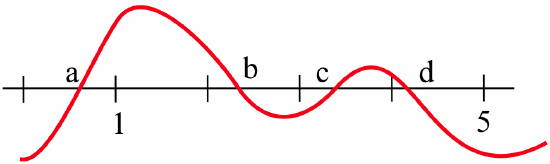
For the function graphed below:

which root do the iterates of Newton’s method approach if:

1. \(x_0 = 2\)?
2. \(x_0 = 3\)?
3. \(x_0 = 5\)?

Answer

The figure below shows the first iteration of Newton’s Method for \(x_0 = 2\), \(3\) and \(5\):

If \(x_0 = 2\), the iterates approach the root at \(a\); if \(x_0 = 3\), they approach the root at \(c\); and if \(x_0 = 5\), they approach the root at \(a\).

Iteration

We have been emphasizing the geometric nature of Newton’s method, but Newton’s method is also an example of iterating a function. If \(\displaystyle N(x) = x - \frac{f(x)}{f'(x)}\), the “pattern” in the algorithm, then: \begin{align*} x_1 &= x_0 - \frac{f(x_0)}{f '(x_0)} = N(x_0) \\ x_2 &= x_1 - \frac{f(x_1)}{f '(x_1)} = N(x_1) = N( N( x_0 ) ) = N\circ N( x_0 )\\ x_3 &= x_2 - \frac{f(x_2)}{f '(x_2)} = N(x_2) = N(N( N( x_0 ) )) = N\circ N\circ N( x_0 ) \end{align*} and, in general:\[x_n = N(x_{n-1}) = n\mbox{th iteration of }N\mbox{ starting with }x_0\nonumber\]At each step, we use the output from \(N\) as the next input into \(N\).

What Can Go Wrong?

When Newton’s method works, it usually works very well and the values of \(x_n\) approach a root of \(f\) very quickly, often doubling the number of correct digits with each iteration. There are, however, several  things that can go wrong.

An obvious problem with Newton’s method is that \(f'(x_n)\) can be \(0\):

Then the algorithm tells us to divide by \(0\) and \(x_{n+1}\) is undefined. Geometrically, if \(f'(x_n) = 0\), the tangent line to the graph of \(f\) at \(x_n\)  is horizontal and does not intersect the \(x\)-axis at any point. If \(f'(x_n) = 0\), just pick another starting value \(x_0\) and begin again. In practice, a second or third choice of \(x_0\) usually succeeds.

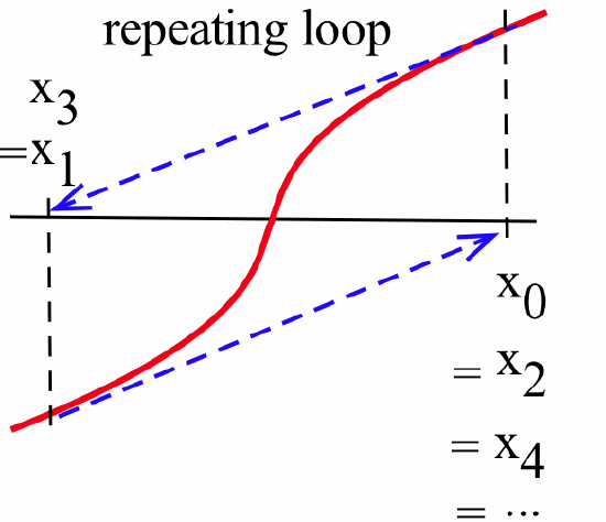
There are two other less obvious difficulties that are not as easy to overcome — the values of the iterates \(x_n\) may become locked into an infinitely repeating loop:

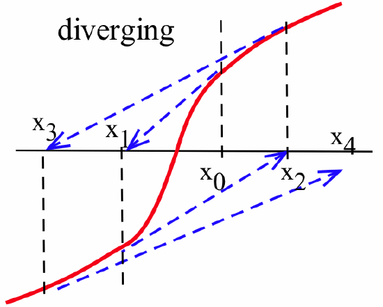
or they may actually move farther away from a root:

Example \(\PageIndex{3}\)

Put \(x_0 = 1\) and use Newton’s method to find the first two iterates, \(x_1\) and \(x_2\), for the function \(f(x) = x^3 - 3x^2 + x - 1\).

Solution

This is the function from the previous Practice Problem, but with a different starting value for \(x_0\): \(f'(x) = 3x^2- 6x + 1\) so, \begin{align*}x_1 &= x_0 - \frac{f(x_0)}{f'(x_0)} = 1 - \frac{f(1)}{f'(1)} = 1 - \frac{-2}{-2} = 0\\ \mbox{and} \ x_2  &= x_1 - \frac{f(x_1)}{f'(x_1)} = 0 - \frac{f(0)}{f'(0)} = 0 - \frac{-1}{1} = 1\end{align*} which is the same as \(x_0\), so \(x_3 = x_1 = 0\) and \(x_4 = x_2 = 1\). The values of \(x_n\) alternate between \(1\) and \(0\) and do not approach a root.

Newton’s method behaves badly at only a few starting points for this particular function — for most starting points, Newton’s method converges to the root of this function. There are some functions, however, that defeat Newton’s method for almost every starting point.

Practice \(\PageIndex{5}\)

For \(\displaystyle f(x) = \sqrt[3]{x} = x^{\frac13}\) and \(x_0 = 1\), verify that \(x_1 = -2\), \(x_2 = 4\) and \(x_3 = -8\). Also try \(x_0 = -3\) and verify that the same pattern holds: \(x_{n+1} = -2x_n\). Graph \(f\) and explain why  the Newton’s method iterates get farther and farther away from the root at \(0\).

Answer

\(f(x) = x^{\frac13} \Rightarrow f'(x) = \frac13 x^{-\frac23}\). If \(x_0 = 1\), then:
\begin{align*}x_1 &= 1 - \frac{f(1)}{f'(1)} = 1 - \frac{1}{\frac13} = 1 - 3 = -2\\
x_2 &= -2 - \frac{f(-2)}{f'(-2)} = -2 - \frac{(-2)^{\frac13}}{\frac13 (-2)^{-\frac23}} = -2 - \frac{-2}{\frac13} = 4\\
x_3 &= 4 - \frac{f(4)}{f'(4)} = 4 - \frac{(4)^{\frac13}}{\frac13 (4)^{-\frac23}} = 4 - \frac{4}{\frac13} = -8\end{align*}
and so on. If \(x_0 = -3\), then:
\begin{align*}x_1 &= -3 - \frac{f(-3)}{f'(-3)} = -3 - \frac{(-3)^{\frac13}}{\frac13 (-3)^{-\frac23}} = -3 + 9  = 6\\
x_2 &= 6 - \frac{f(6)}{f'(6)} = 6 - \frac{(6)^{\frac13}}{\frac13 (6)^{-\frac23}} = 6 - \frac{6}{\frac13} = -12\end{align*}
The graph of \(f(x) = \sqrt[3]{x}\) has a shape similar to the figure below: FIGURE and the behavior of the iterates is similar to the pattern shown in that figure. Unless \(x_0 = 0\) (the only root of \(f\)) the iterates alternate in sign and double in magnitude with each iteration: they get progressively farther from the root with each iteration.

Newton’s method is powerful and quick and very easy to program on a calculator or computer. It usually works so well that many people routinely use it as the first method they apply. If Newton’s method fails for their particular function, they simply try some other method.

Chaotic Behavior and Newton’s Method

An algorithm leads to chaotic behavior if two starting points that are close together generate iterates that are sometimes far apart and sometimes close together: \(\left| a_0 - b_0 \right|\) is small but \(\left| a_n - b_n \right|\) is large for lots (infinitely many) of values of \(n\) and \(\left| a_n - b_n \right|\) is small for lots of values of \(n\). The iterates of the next simple algorithm exhibit chaotic behavior. 

A Simple Chaotic Algorithm: Starting with any number between \(0\) and \(1\), double the number and keep the fractional part of the result: \(x_1\) is the fractional part of \(2x_0\), \(x_2\) is the fractional part of \(2x_1\), and in general, \(x_{n+1} = 2x_n- \left\lfloor 2x_n\right\rfloor\).

If \(x_0 = 0.33\), then the iterates of this algorithm are \(0.66\), \(0.32 =\) fractional part of \(2\cdot 0.66\), \(0.64\), \(0.28\), \(0.56\), … The iterates for two other starting values close to \(0.33\) are given below as well as the iterates of \(0.470\) and \(0.471\):

\(x_0\)	\(0.32\)	\(0.33\)	\(0.34\)	\(0.470\)	\(0.471\)
\(x_1\)	\(0.64\)	\(0.66\)	\(0.68\)	\(0.940\)	\(0.942\)
\(x_2\)	\(0.28\)	\(0.32\)	\(0.36\)	\(0.880\)	\(0.884\)
\(x_3\)	\(0.56\)	\(0.64\)	\(0.72\)	\(0.760\)	\(0.768\)
\(x_4\)	\(0.12\)	\(0.28\)	\(0.44\)	\(0.520\)	\(0.536\)
\(x_5\)	\(0.24\)	\(0.56\)	\(0.88\)	\(0.040\)	\(0.072\)
\(x_6\)	\(0.48\)	\(0.12\)	\(0.76\)	\(0.080\)	\(0.144\)
\(x_7\)	\(0.96\)	\(0.24\)	\(0.56\)	\(0.160\)	\(0.288\)
\(x_8\)	\(0.92\)	\(0.48\)	\(0.12\)	\(0.320\)	\(0.576\)
\(x_9\)	\(0.84\)	\(0.96\)	\(0.24\)	\(0.640\)	\(0.152\)

There are starting values as close together as we want whose iterates are far apart infinitely often.

Many physical, biological and financial phenomena exhibit chaotic behavior. Atoms can start out within inches of each other and several weeks later be hundreds of miles apart. The idea that small initial differences  can lead to dramatically diverse outcomes is sometimes called the “butterfly effect” from the title of a talk (“Predictability: Does the Flap of a Butterfly’s Wings in Brazil Set Off a Tornado in Texas?”) given by Edward Lorenz, one of the first people to investigate chaos. The “butterfly effect” has important implications about the possibility — or rather the impossibility — of accurate long-range weather forecasting. Chaotic behavior is also an important aspect of studying turbulent air and water flows, the incidence and spread of diseases, and even the fluctuating behavior of the stock market.

Newton’s method often exhibits chaotic behavior and — because it is relatively easy to study — is often used as a model to investigate the properties of chaotic behavior. If we use Newton’s method to approximate the roots of \(f(x) = x^3- x\) (with roots \(0\), \(+1\) and \(-1\)), then starting points that are very close together can have iterates that converge to different roots. The iterates of \(0.4472\) and \(0.4473\) converge to the roots \(0\) and \(+1\), respectively. The iterates of the median value \(0.44725\) converge to the root \(-1\), and the iterates of another nearby point, \(\displaystyle \frac{1}{\sqrt{5}} \approx 0.44721\), simply cycle between \(\displaystyle -\frac{1}{\sqrt{5}}\) and \(\displaystyle +\frac{1}{\sqrt{5}}\) and do not converge at all.

Practice \(\PageIndex{6}\)

Find the first four Newton’s method iterates of \(x_0 = 0.997\) and \(x_0 = 1.02\) for \(f(x) = x^2 + 1\). Try two other starting values very close to \(1\) (but not equal to \(1\)) and find their first four iterates. Use the graph of \(f(x) = x^2 + 1\) to explain how starting points so close together can quickly have iterates so far apart.

Answer

If \(x_0 = 0.997\), then \(x_1 \approx -0.003\), \(x_2 \approx 166.4\), \(x_3 \approx 83.2\), \(x_4 \approx 41.6\). If \(x_0 = 1.02\), then \(x_1 \approx 0.0198\), \(x_2 \approx -25.2376\) , \(x_3 \approx -12.6\) and \(x_4 \approx -6.26\).

Problems

1. The graph of \(y = f(x)\) appears below:
   
   Estimate the locations of \(x_1\) and \(x_2\) when you apply Newton’s method with the given starting value \(x_0\).
2. The graph of \(y = g(x)\) appears below:
   
   Estimate the locations of \(x_1\) and \(x_2\) when you apply Newton’s method starting value with the value \(x_0\) shown in the graph.
3. The function graphed below has several roots:
   
   Which root do the iterates of Newton’s method converge to if we start with \(x_0 = 1\)? With \(x_0 = 5\)?
4. The function graphed below has several roots:
   
   Which root do the iterates of Newton’s method converge to if we start with \(x_0 = 2\)? With \(x_0 = 6\)?
5. What happens to the iterates if we apply Newton’s method to the function graphed below:
   
   and start with \(x_0 = 1\)? With \(x_0 = 5\)?
6. What happens if we apply Newton’s method to a function \(f\) and start with \(x_0 =\) a root of \(f\)?
7. What happens if we apply Newton’s method to a function \(f\) and start with \(x_0 =\) a maximum of \(f\)?

In Problems 8–9, a function and a value for \(x_0\) are given. Apply Newton’s method to find \(x_1\) and \(x_2\).

8. \(f(x) = x^3 + x - 1\) and \(x_0 = 1\)
9. \(f(x) = x^4- x^3- 5\) and \(x_0 = 2\)

In Problems 10–11, use Newton’s method to find a root, accurate to 2 decimal places, of the given functions using the given starting points.

10. \(f(x) = x^3- 7\) and \(x_0 = 2\)
11. \(f(x) = x - \cos(x)\) and \(x_0 = 0.7\)

In Problems 12–15, use Newton’s method to find all roots or solutions, accurate to 2 decimal places, of the given equation. It is helpful to examine a graph to determine a “good” starting value \(x_0\).

12. \(2 + x = e^x\)
13. \(\displaystyle \frac{x}{x + 3} = x^2 - 2\)
14. \(x = \sin(x)\)
15. \(x = \sqrt[5]{3}\)
16. Show that if you apply Newton’s method to \(f(x) = x^2 - A\) to approximate \(\sqrt{A}\), then:\[x_{n+1} = \frac12\left(x_n + \frac{A}{x_n}\right)\nonumber\]so the new estimate of the square root is the average of the previous estimate and \(A\) divided by the previous estimate. This method of approximating square roots is called Heron's method.
17. Use Newton’s method to devise an algorithm for approximating the cube root of a number \(A\).
18. Use Newton’s method to devise an algorithm for approximating the \(n\)-th root of a number \(A\).

Problems 19–22 involve chaotic behavior.

19. The iterates of numbers using the Simple Chaotic Algorithm have some interesting properties.
    1. Verify that the iterates starting with \(x_0 = 0\) are all equal to \(0\).
    2. Verify that if \(x_0 = \frac12\), \(\frac14\), \(\frac18\) and, in general, \(\frac{1}{2^n}\), then the \(n\)-th iterate of \(x_0\) is \(0\) (and so are all iterates beyond the \(n\)-th iterate.)
20. When Newton’s method is applied to the function \(f(x) = x^2 + 1\), most starting values for \(x_0\) lead to chaotic behavior for \(x_n\). Find a value for \(x_0\) so that the iterates alternate: \(x_1 = -x_0\) and \(x_2 = -x_1 = x_0\).
21. The function \(f(x)\) defined as:\[f(x) = \left\{ \begin{array}{rl} { 2x } & { \text{if } 0 \leq x < \frac12 } \\ { 2 - 2x } & { \text{if } \frac12 \leq x \leq 1 } \end{array}\right.\nonumber\] is called a “stretch and fold” function.
    1. Describe what \(f\) does to the points in the interval \(\left[0, 1\right]\).
    2. Examine and describe the behavior of the iterates of \(\frac23\), \(\frac25\), \(\frac27\) and \(\frac29\).
    3. Examine and describe the behavior of the iterates of \(0.10\), \(0.105\) and \(0.11\).
    4. Do the iterates of \(f\) lead to chaotic behavior?
22. 1. After many iterations (50 is fine) what happens when you apply Newton’s method starting with \(x_0 = 0.5\) to:
       1. \(f(x) = 2x(1-x)\)
       2. \(f(x) = 3.3x(1-x)\)
       3. \(f(x) = 3.83x(1-x)\)
    2. What do you think happens to the iterates of \(f(x) = 3.7x(1-x)\)? What actually happens?
    3. Repeat parts (a)–(b) with some other starting values \(x_0\) between \(0\) and \(1\) (\(0 < x_0 < 1\)).
    (The behavior of the iterates of \(f\) depends in a strange way on the numerical value of the leading coefficient. The behavior exhibited in part (b) is an example of “chaos.”)