
2.8: Linear Approximation and Differentials
- Page ID
- 212018

\( \newcommand{\vecs}[1]{\overset { \scriptstyle \rightharpoonup} {\mathbf{#1}} } \)
\( \newcommand{\vecd}[1]{\overset{-\!-\!\rightharpoonup}{\vphantom{a}\smash {#1}}} \)
\( \newcommand{\dsum}{\displaystyle\sum\limits} \)
\( \newcommand{\dint}{\displaystyle\int\limits} \)
\( \newcommand{\dlim}{\displaystyle\lim\limits} \)
\( \newcommand{\id}{\mathrm{id}}\) \( \newcommand{\Span}{\mathrm{span}}\)
( \newcommand{\kernel}{\mathrm{null}\,}\) \( \newcommand{\range}{\mathrm{range}\,}\)
\( \newcommand{\RealPart}{\mathrm{Re}}\) \( \newcommand{\ImaginaryPart}{\mathrm{Im}}\)
\( \newcommand{\Argument}{\mathrm{Arg}}\) \( \newcommand{\norm}[1]{\| #1 \|}\)
\( \newcommand{\inner}[2]{\langle #1, #2 \rangle}\)
\( \newcommand{\Span}{\mathrm{span}}\)
\( \newcommand{\id}{\mathrm{id}}\)
\( \newcommand{\Span}{\mathrm{span}}\)
\( \newcommand{\kernel}{\mathrm{null}\,}\)
\( \newcommand{\range}{\mathrm{range}\,}\)
\( \newcommand{\RealPart}{\mathrm{Re}}\)
\( \newcommand{\ImaginaryPart}{\mathrm{Im}}\)
\( \newcommand{\Argument}{\mathrm{Arg}}\)
\( \newcommand{\norm}[1]{\| #1 \|}\)
\( \newcommand{\inner}[2]{\langle #1, #2 \rangle}\)
\( \newcommand{\Span}{\mathrm{span}}\) \( \newcommand{\AA}{\unicode[.8,0]{x212B}}\)
\( \newcommand{\vectorA}[1]{\vec{#1}} % arrow\)
\( \newcommand{\vectorAt}[1]{\vec{\text{#1}}} % arrow\)
\( \newcommand{\vectorB}[1]{\overset { \scriptstyle \rightharpoonup} {\mathbf{#1}} } \)
\( \newcommand{\vectorC}[1]{\textbf{#1}} \)
\( \newcommand{\vectorD}[1]{\overrightarrow{#1}} \)
\( \newcommand{\vectorDt}[1]{\overrightarrow{\text{#1}}} \)
\( \newcommand{\vectE}[1]{\overset{-\!-\!\rightharpoonup}{\vphantom{a}\smash{\mathbf {#1}}}} \)
\( \newcommand{\vecs}[1]{\overset { \scriptstyle \rightharpoonup} {\mathbf{#1}} } \)
\(\newcommand{\longvect}{\overrightarrow}\)
\( \newcommand{\vecd}[1]{\overset{-\!-\!\rightharpoonup}{\vphantom{a}\smash {#1}}} \)
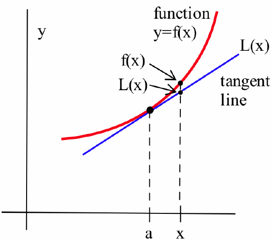
\(\newcommand{\avec}{\mathbf a}\) \(\newcommand{\bvec}{\mathbf b}\) \(\newcommand{\cvec}{\mathbf c}\) \(\newcommand{\dvec}{\mathbf d}\) \(\newcommand{\dtil}{\widetilde{\mathbf d}}\) \(\newcommand{\evec}{\mathbf e}\) \(\newcommand{\fvec}{\mathbf f}\) \(\newcommand{\nvec}{\mathbf n}\) \(\newcommand{\pvec}{\mathbf p}\) \(\newcommand{\qvec}{\mathbf q}\) \(\newcommand{\svec}{\mathbf s}\) \(\newcommand{\tvec}{\mathbf t}\) \(\newcommand{\uvec}{\mathbf u}\) \(\newcommand{\vvec}{\mathbf v}\) \(\newcommand{\wvec}{\mathbf w}\) \(\newcommand{\xvec}{\mathbf x}\) \(\newcommand{\yvec}{\mathbf y}\) \(\newcommand{\zvec}{\mathbf z}\) \(\newcommand{\rvec}{\mathbf r}\) \(\newcommand{\mvec}{\mathbf m}\) \(\newcommand{\zerovec}{\mathbf 0}\) \(\newcommand{\onevec}{\mathbf 1}\) \(\newcommand{\real}{\mathbb R}\) \(\newcommand{\twovec}[2]{\left[\begin{array}{r}#1 \\ #2 \end{array}\right]}\) \(\newcommand{\ctwovec}[2]{\left[\begin{array}{c}#1 \\ #2 \end{array}\right]}\) \(\newcommand{\threevec}[3]{\left[\begin{array}{r}#1 \\ #2 \\ #3 \end{array}\right]}\) \(\newcommand{\cthreevec}[3]{\left[\begin{array}{c}#1 \\ #2 \\ #3 \end{array}\right]}\) \(\newcommand{\fourvec}[4]{\left[\begin{array}{r}#1 \\ #2 \\ #3 \\ #4 \end{array}\right]}\) \(\newcommand{\cfourvec}[4]{\left[\begin{array}{c}#1 \\ #2 \\ #3 \\ #4 \end{array}\right]}\) \(\newcommand{\fivevec}[5]{\left[\begin{array}{r}#1 \\ #2 \\ #3 \\ #4 \\ #5 \\ \end{array}\right]}\) \(\newcommand{\cfivevec}[5]{\left[\begin{array}{c}#1 \\ #2 \\ #3 \\ #4 \\ #5 \\ \end{array}\right]}\) \(\newcommand{\mattwo}[4]{\left[\begin{array}{rr}#1 \amp #2 \\ #3 \amp #4 \\ \end{array}\right]}\) \(\newcommand{\laspan}[1]{\text{Span}\{#1\}}\) \(\newcommand{\bcal}{\cal B}\) \(\newcommand{\ccal}{\cal C}\) \(\newcommand{\scal}{\cal S}\) \(\newcommand{\wcal}{\cal W}\) \(\newcommand{\ecal}{\cal E}\) \(\newcommand{\coords}[2]{\left\{#1\right\}_{#2}}\) \(\newcommand{\gray}[1]{\color{gray}{#1}}\) \(\newcommand{\lgray}[1]{\color{lightgray}{#1}}\) \(\newcommand{\rank}{\operatorname{rank}}\) \(\newcommand{\row}{\text{Row}}\) \(\newcommand{\col}{\text{Col}}\) \(\renewcommand{\row}{\text{Row}}\) \(\newcommand{\nul}{\text{Nul}}\) \(\newcommand{\var}{\text{Var}}\) \(\newcommand{\corr}{\text{corr}}\) \(\newcommand{\len}[1]{\left|#1\right|}\) \(\newcommand{\bbar}{\overline{\bvec}}\) \(\newcommand{\bhat}{\widehat{\bvec}}\) \(\newcommand{\bperp}{\bvec^\perp}\) \(\newcommand{\xhat}{\widehat{\xvec}}\) \(\newcommand{\vhat}{\widehat{\vvec}}\) \(\newcommand{\uhat}{\widehat{\uvec}}\) \(\newcommand{\what}{\widehat{\wvec}}\) \(\newcommand{\Sighat}{\widehat{\Sigma}}\) \(\newcommand{\lt}{<}\) \(\newcommand{\gt}{>}\) \(\newcommand{\amp}{&}\) \(\definecolor{fillinmathshade}{gray}{0.9}\)Newton’s method used tangent lines to “point toward” a root of a function. In this section we examine and use another geometric characteristic of tangent lines:
If: \(f\) is differentiable at \(a\), \(c\) is close to \(a\)
and: \(y = L(x)\) is the line tangent to \(f(x)\) at \(x = a\)
then: \(L(c)\) is close to \(f(c)\).
We can use this idea to approximate the values of some commonly used functions and to predict the “error” or uncertainty in a computation if we know the “error” or uncertainty in our original data. At the end of this section, we will define a related concept called the differential of a function.
Linear Approximation
Because this section uses tangent lines extensively, it is worthwhile to recall how we find the equation of the line tangent to \(f(x)\) where \(x=a\): the tangent line goes through the point \((a, f(a))\) and has slope \(f'(a)\) so, using the point-slope form \(y - y_0 = m(x - x_0)\) for linear equations, we have \(y - f(a) = f'(a)\cdot (x - a) \ \Rightarrow \ y = f(a) + f '(a)\cdot (x - a)\).
If: \(f\) is differentiable at \(x = a\)
then: an equation of the line \(L\) tangent to \(f\) at \(x = a\) is \(L(x) = f(a) + f '(a)\cdot (x - a)\)
Find a formula for \(L(x)\), the linear function tangent to the graph of \(f(x) = \sqrt{x}\) at the point \((9,3)\).

Evaluate \(L(9.1)\) and \(L(8.88)\) to approximate \(\sqrt{9.1}\) and \(\sqrt{8.88}\).
Solution
\(f(x) = \sqrt{x} = x^{\frac12} \Rightarrow f'(x) = \frac12 x^{-\frac12} = \frac{1}{2\sqrt{x}}\) so \(f(9) = 3\) and \(f'(9) = \frac{1}{2\sqrt{9}} = \frac16\). Thus:\[L(x) = f(9) + f'(9)\cdot (x - 9) = 3 + \frac16 (x - 9)\nonumber\]If \(x\) is close to \(9\), then the value of \(L(x)\) should be a good approximation of the value of \(x\). The number \(9.1\) is close to \(9\) so \(\sqrt{9.1} = f(9.1) \approx L(9.1) = 3 + \frac16 (9.1 - 9) \approx 3.016666\). Similarly, \(\sqrt{8.88} = f(8.88) \approx L(8.88) = 3 + \frac16 (8.88 - 9) = 2.98\). In fact, \(\sqrt{9.1} \approx 3.016621\), so our estimate using \(L(9.1)\) is within \(0.000045\) of the exact answer; \(\sqrt{8.88} \approx 2.979933\) (accurate to 6 decimal places) and our estimate is within \(0.00007\) of the exact answer.
In each case in the previous example, we got a good estimate of a square root with very little work. The graph in the margin indicates the graph of the tangent line \(y = L(x)\) lies slightly above the graph of \(y = f(x)\); consequently (as we observed), each estimate is slightly larger than the exact value.
Find a formula for \(L(x)\), the linear function tangent to the graph of \(f(x) = \sqrt{x}\) at the point \((16,4)\). Evaluate \(L(16.1)\) and \(L(15.92)\) to approximate \(\sqrt{16.1}\) and \(\sqrt{15.92}\).

Are your approximations using \(L\) larger or smaller than the exact values of the square roots?
- Answer
-
\(f(x) = x^{\frac12} \Rightarrow f'(x) = \frac{1}{2\sqrt{x}}\). At the point \((16,4)\) on the graph of \(f\), the slope of the tangent line is \(f'(16) = \frac{1}{2\sqrt{16}} = \frac{1}{8}\). An equation of the tangent line is \(y - 4 = \frac18 (x - 16)\) or \(y = \frac18 x + 2\): \(L(x) = \frac18 x + 2\). So:
\begin{align*}\sqrt{16.1} &\approx L(16.1) = \frac18 (16.1) + 2 = 4.0125\\
\sqrt{15.92} &\approx L(15.92) = \frac18 (15.92) + 2 = 3.99\end{align*}
FInd a formula for \(L(x)\), the linear function tangent to the graph of \(f(x) = x^3\) at the point \((1,1)\) and use \(L(x)\) to approximate \((1.02)^3\) and \((0.97)^3\). Do you think your approximations using \(L\) are larger or smaller than the exact values?
- Answer
-
\(f(x) = x^3 \Rightarrow f'(x) = 3x^2\). At \((1,1)\), the slope of the tangent line is \(f'(1) = 3\). An equation of the tangent line is \(y - 1 = 3(x - 1)\) or \(y = 3x - 2\): \(L(x) = 3x - 2\). So:
\begin{align*}(1.02)^3 &\approx L(1.02) = 3(1.02) - 2 = 1.06\\
(0.97)^3 &\approx L(0.97) = 3(0.97) - 2 = 0.91\end{align*}
The process we have used to approximate square roots and cubics can be used to approximate values of any differentiable function, and the main result about the linear approximation follows from the two statements in the boxes. Putting these two statements together, we have the process for Linear Approximation.
If: \(f\) is differentiable at \(a\) and \(L(x) = f(a) + f'(a)\cdot (x - a)\)
then: (geometrically) the graph of \(L(x)\) is close to the graph of \(f(x)\) when \(x\) is close to \(a\)
and: (algebraically) the values of the \(L(x)\) approximate the values of \(f(x)\) when \(x\) is close to \(a\):\[f(x) \approx L(x) = f(a) + f'(a)\cdot (x - a)\nonumber\]
Sometimes we replace “\(x - a\)” with “\(\Delta x\)” in the last equation, and the statement becomes \(f(x) \approx f(a) + f '(a)\cdot \Delta x\).

Use the linear approximation process to approximate the value of \(e^{0.1}\).
Solution
\(f(x) = e^x \Rightarrow f'(x) = e^x\) so we need to pick a value \(a\) near \(x = 0.1\) for which we know the exact value of \(f(a) = e^a\) and \(f'(a) = e^a\): \(a = 0\) is an obvious choice. Then:
\begin{align*}
e^{0.1} &= f(0.1) \approx L(0.1) = f(0) + f'(0)\cdot (0.1 - 0)\\
&= e^0 + e^0\cdot (0.1) = 1 + 1\cdot (0.1) = 1.1\end{align*}
You can use your calculator to verify that this approximation is within \(0.0052\) of the exact value of \(e^{0.1}\).
Approximate the value of \((1.06)^4\), the amount $1 becomes after 4 years in a bank account paying 6% interest compounded annually. (Take \(f(x) = x^4\) and \(a = 1\).)
- Answer
-
\(f(x) = x^4 \Rightarrow f'(x) = 4x^3\). Taking \(a = 1\) and \(\Delta x = 0.06\):
\begin{align*}(1.06)^4 &= f(1.06) \approx L(1.06) = f(1) + f'(1)\cdot (0.06)\\
&= 1^4 + 4(1^3)(0.06) = 1.24\end{align*}
Use the linear approximation process and the values in the table below to estimate the value of \(f\) when \(x = 1.1\), \(1.23\) and \(1.38\).
| \(x\) | \(f(x)\) | \(f'(x)\) |
|---|---|---|
| \(1.0\) | \(0.7854\) | \(0.5\) |
| \(1.2\) | \(0.8761\) | \(0.4098\) |
| \(1.4\) | \(0.9505\) | \(0.3378\) |
- Answer
-
Using values given in the table:
\begin{align*}f(1.1) &\approx f(1) + f '(1)\cdot (0.1)\\
&= 0.7854 + (0.5)(0.1) = 0.8354\\
f(1.23) &\approx f(1.2) + f'(1.2)\cdot (0.03)\\
&= 0.8761 + (0.4098)(0.03) = 0.888394\\
f(1.38) &\approx f(1.4) + f'(1.4)\cdot (-0.02)\\ &= 0.9505 + (0.3378)(-0.02) = 0.943744\end{align*}
We can approximate functions as well as numbers (specific values of those functions).
Find a linear approximation formula \(L(x)\) for \(\sqrt{1 + x}\) when \(x\) is small. Use your result to approximate \(\sqrt{1.1}\) and \(\sqrt{0.96}\).
Solution
\(f(x) = \sqrt{1 + x} = (1 + x)^{\frac12} \Rightarrow f'(x) = \frac12 (1 + x)^{-\frac12} = \frac{1}{2\sqrt{1+x}}\), so because “\(x\) is small,” we know that \(x\) is close to \(0\) and we can pick \(a = 0\). Then \(f(a) = f(0) = 1\) and \(f'(a) = f'(0) = \frac12\) so\[\sqrt{1 + x} \approx L(x) = f(0) + f'(0)\cdot (x - 0) = 1 + \frac12 x = 1 + \frac{x}{2}\nonumber\]Taking \(x= 0.1\), \(\sqrt{1.1} =\sqrt{1+0.1} \approx 1 + \frac{0.1}{2}= 1.05\); taking \(x = -0.04\), \(\sqrt{0.96} = \sqrt{1 + (-.04)} \approx 1 + \frac{-0.04}{2} = 0.98\). Use your calculator to determine by how much each estimate differs from the true value.
Applications of Linear Approximation to Measurement “Error”
Most scientific experiments use instruments to take measurements, but these instruments are not perfect, and the measurements we get from them are only accurate up to a certain level of precision. If we know this level of accuracy of our instruments and measurements, we can use the idea of linear approximation to estimate the level of accuracy of results we calculate from our measurements.
If we measure the side \(x\) of a square to be 8 inches, then we would of course calculate its area to be \(8^2= 64\) square inches. Suppose, as would reasonable with a real measurement, that our measuring instrument could only measure or be read to the nearest 0.05 inches. Then our measurement of 8 inches would really mean some number between \(8-0.05 = 7.95\) inches and \(8+0.05 = 8.05\) inches, so the true area of the square would be between \(7.95^2 = 63.2025\) and \(8.05^2 = 64.8025\) square inches. Our possible “error” or “uncertainty,” because of the limitations of the instrument, could be as much as \(64.8025 - 64 = 0.8025\) square inches, so we could report the area of the square to be \(64 \pm 0.8025\) square inches. We can also use the linear approximation method to estimate the “error” or uncertainty of the area. (For a function as simple as the area of a square, this linear approximation method really isn't needed, but it serves as a useful and easily understood illustration of the technique.)
For a square with side \(x\), the area is \(A(x) = x^2\) and \(A'(x) = 2x\). If \(\Delta x\) represents the “error” or uncertainty of our measurement of the side then, using the linear approximation technique for \(A(x)\), \(A(x) \approx A(a) + A'(a)\cdot \Delta x\) so the uncertainty of our calculated area is \(A(x ) - A(a) \approx A'(a)\cdot \Delta x\). In this example, \(a = 8\) inches and \(\Delta x = 0.05\) inches, so \(A(8.05) \approx A(8) + A'(8)\cdot (0.05) = 64 + 2(8)\cdot (0.05) = 64.8\) square inches, and the uncertainty in our calculated area is approximately \(A(8 + 0.05) - A(8) \approx A'(8)\cdot \Delta x = 2(8\mbox{ inches})(0.05\mbox{ inches}) = 0.8\) square inches. (Compare this approximation of the biggest possible error with the exact answer of \(0.8025\) square inches computed previously.) This process can be summarized as:
If: the value of the \(x\)-variable is measured to be \(x = a\) with a maximum “error” of \(\Delta x\) units
then: \(\Delta f\), the “error” in estimating \(f(x)\), is:\[\Delta f = f(x) - f(a) \approx f'(a)\cdot \Delta x\nonumber\]
If we measure the side of a cube to be 4 cm with an uncertainty of 0.1 cm, what is the volume of the cube and the uncertainty of our calculation of the volume? (Use linear approximation.)
- Answer
-
\(f(x) = x^3 \Rightarrow f'(x) = 3x^2\) so \(f(4) = 4^3 = 64\) cm\(^3\) and the “error” is:\[\Delta f \approx f'(x)\cdot \Delta x = 3x^2 \cdot \Delta x\nonumber\]When \(x = 4\) and \(\Delta x = 0.1\), \(\Delta f \approx 3(4)^2(0.1) = 4.8\) cm\(^3\).
We are using a tracking telescope to follow a small rocket. Suppose we are 3,000 meters from the launch point of the rocket, and, 2 seconds after the launch we measure the angle of the inclination of the rocket to be 64\(^{\circ}\) with a possible “error” of 2\(^{\circ}\).

How high is the rocket and what is the possible error in this calculated height?
Solution
Our measured angle is \(x = 1.1170\) radians with \(\Delta x = 0.0349\) radians (all trigonometric work should be in radians), and the height of the rocket at an angle \(x\) is \(f(x) = 3000\tan( x )\) so \(f(1.1170) \approx 6151\) m. Our uncertainty in the height is \(\Delta f \approx f'(x)\cdot \Delta x \approx 3000\cdot \sec^2(x) \cdot \Delta x = 3000\sec^2(1.1170)\cdot 0.0349 \approx 545\) m. If our measured angle of 64\(^{\circ}\) can be in error by as much as 2\(^{\circ}\), then our calculated height of 6,151 m can be in error by as much as 545 m. The height is \(6151 \pm 545\) meters
Suppose we measured the angle of inclination in the previous Example to be \(43^{\circ} \pm 1^{\circ}\). Estimate the height of the rocket in the form “height \(\pm\) error.”
- Answer
-
\(43^{\circ} \pm 1^{\circ}\) is equivalent to \(0.75049 \pm 0.01745\) radians, so with \(f(x) = 3000\tan(x)\) we have \(f(0.75049) = 3000\tan(0.75049) \approx 2797.5\) m and \(f'(x) = 3000\sec^2(x)\). So:
\begin{align*}\Delta f &\approx f '(x)\cdot \Delta x = 3000\sec^2(x)\cdot \Delta x\\ &= 3000\sec^2(0.75049)\cdot (0.01745) = 97.9 \mbox{ m}\end{align*}
The height of the rocket is \(2797.5 \pm 97.9\) m.
In some scientific and engineering applications, the calculated result must be within some given specification. You might need to determine how accurate the initial measurements must be in order to guarantee the final calculation is within that specification. Added precision usually costs time and money, so it is important to choose a measuring instrument good enough for the job but which is not too expensive.
Your company produces ball bearings (small metal spheres) with a volume of 10 cm\(^3\) and the volume must be accurate to within 0.1 cm\(^3\). What radius should the bearings have — and what error can you tolerate in the radius measurement to meet the accuracy specification for the volume?
Solution
We want \(V = 10\) and we know that the volume of a sphere is \(V = \frac43 \pi r^3\), so solve \(10 = \frac43\pi r^3\) for \(r\) to get \(r = 1.3365\) cm. \(V(r) = \frac43\pi r^3 \Rightarrow V'(r) = 4\pi r^2\) so \(\Delta V \approx V'(r) \cdot \Delta r\). In this case we know that \(\Delta V = 0.1\) cm\(^3\) and we have calculated \(r = 1.3365\) cm, so \(0.1\mbox{ cm}^3 = V'(1.3365\mbox{ cm})\cdot\Delta r = (22.45\mbox{ cm}^2)\cdot\Delta r\). Solving for \(\Delta r\), we get \(\Delta r \approx 0.0045\) cm. To meet the specification for allowable error in volume, we must allow the radius to vary no more than \(0.0045\) cm. If we instead measure the diameter of the sphere, then we want the diameter to be \(d = 2r = 2(1.3365 \pm 0.0045) = 2.673 \pm 0.009\) cm.
You want to determine the height of a rocket to within 10 meters when it is 4,000 meters high:
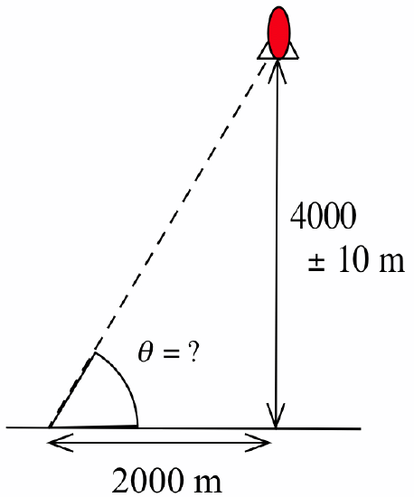
How accurate must your angle of measurement be? (Do your calculations in radians.)
- Answer
-
\(f(\theta) = 2000\tan(\theta) \Rightarrow f'(\theta) = 2000\sec^2(\theta)\) and we know \(f(\theta) = 4000\), so:\[4000 = 2000\tan(\theta) \Rightarrow \tan(\theta) = 2 \Rightarrow \theta \approx 1.10715\mbox{ (radians)}\nonumber\]and thus \(f'(1.10715) = 2000\sec^2(1.10715) \approx 10000\). Finally, the “error” is given by \(\Delta f \approx f'(\theta)\cdot \Delta \theta\) so:\[10 \approx 10000\cdot \Delta \theta \ \Rightarrow \ \Delta \theta \approx \frac{10}{10000} = 0.001\mbox{ (radians) } \approx 0.057^{\circ}\nonumber\]
Relative Error and Percentage Error
The “error” we’ve been examining is called the absolute error to distinguish it from two other commonly used terms, the relative error and the percentage error, which compare the absolute error with the magnitude of the number being measured. An “error” of 6 inches in measuring the Earth's circumference would be extremely small, but a 6-inch error in measuring your head for a hat would result in a very bad fit.
The Relative Error of \(f\) is: \(\displaystyle \frac{\mbox{error of }f}{\mbox{value of }f} = \frac{\Delta f}{f}\)\\ \vspace{0.25cm}
The Percentage Error of \(f\) is: \(\displaystyle \frac{\Delta f}{f}\cdot100\%\).
If the relative error in the calculation of the area of a circle must be less than \(0.4\), then what relative error can we tolerate in the measurement of the radius?
Solution
\(A(r) = \pi r^2 \Rightarrow A'(r) = 2\pi r\) and \(\Delta A \approx A'(r)\cdot \Delta r = 2\pi r \Delta r\). The Relative Error of \(A\) is:\[\frac{\Delta A}{A} \approx \frac{2\pi r \Delta r}{\pi r^2} = 2 \frac{\Delta r}{r}\nonumber\]We can guarantee that the Relative Error of \(A\), \(\displaystyle \frac{\Delta A}{A}\), is less than \(0.4\) if the Relative Error of \(r\), \(\displaystyle \frac{\Delta r}{r} = \frac12 \frac{\Delta A}{A}\), is less than \(\frac12(0.4) = 0.2\).
If you can measure the side of a cube with a percentage error less than 3%, then what will the percentage error for your calculation of the surface area of the cube be?
- Answer
-
\(A(r) = 6r^2 \Rightarrow A'(r) = 12r \Rightarrow \Delta A \approx A'(r)\cdot \Delta r = 12r\cdot\Delta r\) and we also know that \(\frac{\Delta r}{r} < 0.03\), so the percentage error is:\[\frac{\Delta A}{A} \cdot 100\% = \frac{12r\cdot \Delta r}{6r^2}\cdot 100\% = \frac{2 \Delta r}{r} \cdot 100 \% < 200(0.03) \% = 6\%\nonumber\]
The Differential of \(f\)
As shown in the figure below, the change in value of the function \(f\) near the point \((x, f(x))\) is \(\Delta f = f(x + \Delta x) - f(x)\) and the change along the tangent line is \(f'(x)\cdot \Delta x\):

If \(\Delta x\) is small, then we have used the approximation that \(\Delta f \approx f '(x)\cdot \Delta x\). This leads to the definition of a new quantity, \(df\), called the differential of \(f\).
The differential of \(f\) is \(df = f'(x)\cdot dx\) where \(dx\) is any real number.
The differential of \(f\) represents the change in \(f\), as \(x\) changes from \(x\) to \(x + dx\), along the tangent line to the graph of \(f\) at the point \((x, f(x))\). If we take \(dx\) to be the number \(\Delta x\), then the differential is an approximation of \(\Delta f\): \(\Delta f \approx f'(x)\cdot \Delta x = f'(x)\cdot dx = df\).
Determine the differential for the functions \(f(x) = x^3- 7x\), \(g(x) = \sin(x)\) and \(h(r) = \pi r^2\).
Solution
\(df = f'(x)\cdot dx = (3x^2- 7)\, dx\), \(dg = g'(x)\cdot dx = \cos(x)\, dx\), and \(dh = h'(r)\, dr = 2\pi r \, dr\).
Determine the differentials of \(f(x) = \ln( x )\), \(u = \sqrt{1 - 3x}\) and \(r = 3 \cos( \theta )\). (While we will do very little with differentials for a while, we will use them extensively in integral calculus.)
- Answer
-
Computing differentials:
\begin{align*}df &= f'(x)\cdot dx = \frac{1}{x} \, dx\\
du &= \frac{du}{dx} \cdot dx = \frac{-3}{2\sqrt{1 - 3x}} \, dx\\
dr &= \frac{dr}{d\theta} \, d\theta = -3 \sin(\theta) \, d\theta\end{align*}
The Linear Approximation “Error” \(\left| f(x) - L(x) \right|\)
An approximation is most valuable if we also have have some measure of the size of the “error,” the distance between the approximate value and the value being approximated. Typically, we will not know the exact value of the error (why not?), but it is useful to know an upper bound for the error. For example, if one scale gives the weight of a gold pendant as 10.64 grams with an error less than 0.3 grams (\(10.64 \pm 0.3\) grams) and another scale gives the weight of the same pendant as 10.53 grams with an error less than 0.02 grams (\(10.53 \pm 0.02\) grams), then we can have more faith in the second approximate weight because of the smaller “error” guarantee. Before finding a guarantee on the size of the error of the linear approximation process, we will check how well the linear approximation process approximates values of some functions we can compute exactly. Then we will prove one bound on the possible error and state a somewhat stronger bound.
Given the function \(f(x) = x^2\), evaluate the expressions \(f(2+\Delta x)\), \(L(2+\Delta x)\) and \(\left| f(2+\Delta x) - L(2+\Delta x) \right|\) for \(\Delta x = 0.1\), \(0.05\), \(0.01\), \(0.001\) and for a general value of \(\Delta x\).
Solution
\(f(2+\Delta x) = (2+\Delta x)^2 = 2^2 + 4\Delta x + (\Delta x)^2\) and \(L(2+\Delta x) = f(2) + f'(2)\cdot \Delta x = 2^2 + 4\cdot \Delta x\). Then:
| \(\Delta x\) | \(f(2+\Delta x)\) | \(L(2+\Delta x)\) | \(\left| f(2+\Delta x) - L(2+\Delta x) \right|\) |
|---|---|---|---|
| \(0.1\) | \(4.41\) | \(4.4\) | \(0.01\) |
| \(0.05\) | \(4.2025\) | \(4.2\) | \(0.0025\) |
| \(0.01\) | \(4.0401\) | \(4.04\) | \(0.0001\) |
| \(0.001\) | \(4.004001\) | \(4.004\) | \(0.000001\) |
Cutting the value of \(\Delta x\) in half makes the error one fourth as large. Cutting \(\Delta x\) to \(\frac{1}{10}\) as large makes the error \(\frac{1}{100}\) as large. In general:
\begin{align*}\left| f(2+\Delta x) - L(2+\Delta x) \right| &= \left| \left(2^2 + 4\cdot \Delta x + (\Delta x)^2\right) - \left(2^2 + 4\cdot \Delta x\right) \right|\\
&= \left(\Delta x\right)^2\end{align*}
This function and error also have a nice geometric interpretation:

\(f(x) = x^2\) is the area of a square of side \(x\) so \(f(2+\Delta x)\) is the area of a square of side \(2+\Delta x\), and that area is the sum of the pieces with areas \(2^2\), \(2\cdot\Delta x\), \(2\cdot\Delta x\) and \((\Delta x)^2\). The linear approximation \(L(2+\Delta x) = 2^2 + 4\cdot \Delta x\) to the area of the square includes the three largest pieces, \(2^2\), \(2\cdot\Delta x\) and \(2\cdot\Delta x\), but omits the small square with area \((\Delta x)^2\) so the approximation is in error by the amount \((\Delta x)^2\).
Given \(f(x) = x^3\), evaluate \(f(4+\Delta x)\), \(L(4+\Delta x)\) and \(\left| f(4+\Delta x) - L(4+\Delta x) \right|\) for \(\Delta x = 0.1\), \(0.05\), \(0.01\), \(0.001\) and for a general value of \(\Delta x\). Use the figure below:

to give a geometric interpretation of \(f(4+\Delta x)\), \(L(4+\Delta x)\) and \(\left| f(4+\Delta x) - L(4+\Delta x) \right|\).
- Answer
-
\(f(x) = x^3 \Rightarrow f'(x) = 3x^2\) so:\[L(4 + \Delta x) = f(4) + f'(4) \Delta x = 4^3 + 3(4)^2 \Delta x = 64 + 48\Delta x\nonumber\]Evaluating the various quantities at the indicated points:
\(\Delta x\) \(f(4 + \Delta x)\) \(L(4 + \Delta x)\) \(\left| f(4+\Delta x) - L(4+\Delta x) \right|\) \(0.1\) \(68.921\) \(68.8\) \(0.121\) \(0.05\) \(66.430125\) \(66.4\) \(0.030125\) \(0.01\) \(64.481201\) \(64.48\) \(0.001201\) \(0.001\) \(64.048012\) \(64.048\) \(0.000012\) \(f(4+\Delta x)\) is the actual volume of the cube with side length \(4+\Delta x\).
\(L(4+\Delta x)\) is the volume of the cube with side length \(4\) (\(V = 64\)) plus the volume of the three “slabs” (\(V = 3\cdot 4^2\cdot\Delta x\)).
\(\left| f(4+\Delta x)-L(4+\Delta x) \right|\) is the volume of the “leftover” pieces from \(L\): the three “rods” (\(V = 3\cdot 4 \cdot (\Delta x)^2\)) and the tiny cube (\(V = (\Delta x)^3\)).
In the previous Example and previous Practice problem, the error \(\left| f(a+\Delta x) - L(a+\Delta x) \right|\) was very small, proportional to \(\left(\Delta x\right)^2\), when \(\Delta x\) was small. In general, this error approaches \(0\) as \(\Delta x \rightarrow 0\).
If: \(f(x)\) is differentiable at \(a\)
and: \(L(a+\Delta x) = f(a) + f'(a)\cdot \Delta x\)
then: \(\displaystyle \lim_{\Delta x\to 0} \, \left| f(a+\Delta x) - L(a+\Delta x) \right| = 0\)
and: \(\displaystyle \lim_{\Delta x \to 0} \, \frac{\left| f(a+\Delta x) - L(a+\Delta x) \right|}{\Delta x} = 0\).\\
Proof
First rewrite the quantity inside the absolute value as:
\begin{align*}f(a+\Delta x) - L(a+\Delta x) &= f(a+\Delta x) - f(a) - f'(a)\cdot \Delta x\\
&= \left[\frac{ f(a+\Delta x) - f(a)}{\Delta x} - f'(a) \right]\cdot \Delta x\end{align*}
But \(f\) is differentiable at \(x=a\) so \(\displaystyle \lim_{\Delta x\to 0} \, \frac{f(a+\Delta x) - f(a)}{\Delta x} = f'(a)\), which we can rewrite as \(\displaystyle \lim_{\Delta x\to 0} \, \left[\frac{f(a+\Delta x) - f(a)}{\Delta x} - f'(a)\right] = 0\). Thus:\[\lim_{\Delta x\to 0} \, \left[ f(a+\Delta x) - L(a+\Delta x) \right] = \lim_{\Delta x\to 0} \, \left[\frac{f(a+\Delta x) - f(a)}{\Delta x} - f'(a)\right]\cdot \lim_{\Delta x \to 0} \, \Delta x = 0\cdot 0 = 0\nonumber\]Not only does the difference \(f(a+ \Delta x) - L(a+ \Delta x)\) approach \(0\), but this difference approaches \(0\) so fast that we can divide it by \(\Delta x\), another quantity approaching \(0\), and the quotient still approaches \(0\).
In the next chapter we will be able to prove that the error of the linear approximation process is in fact proportional to \((\Delta x)^2\). For now, we just state the result.
If: \(f\) is differentiable at \(a\)
and: \(\left|f ''(x) \right| \leq M\) for all \(x\) between \(a\) and \(a+\Delta x\)
then: \(\left|\mbox{“error”}\right| = \left| f(a+\Delta x) - L(a+\Delta x) \right| \leq \frac12 M\cdot (\Delta x)^2\).
Problems
- The figure below shows the tangent line to a function \(g\) at the point \((2,2)\) and a line segment \(\Delta x\) units long:

- On the figure, label the locations of
- \(2 + \Delta x\) on the \(x\)-axis
- the point \(( 2 + \Delta x, g(2 + \Delta x) )\)
- the point \((2 + \Delta x, g(2) + g'(2)\cdot \Delta x)\)
- How large is the “error,” \((g(2) + g'(2)\cdot \Delta x) - ( g(2+\Delta x) )\)?
- On the figure, label the locations of
- In the figure below, is the linear approximation \(L(a + \Delta x)\) larger or smaller than the value of \(f(a + \Delta x)\) when:

- \(a = 1\) and \(\Delta x = 0.2\)?
- \(a = 2\) and \(\Delta x = -0.1\)?
- \(a = 3\) and \(\Delta x = 0.1\)?
- \(a = 4\) and \(\Delta x = 0.2\)?
- \(a = 4\) and \(\Delta x = -0.2\)?
In Problems 3–4, find a formula for the linear function \(L(x)\) tangent to the given function \(f\) at the given point \((a, f(a))\). Use the value \(L(a + \Delta x)\) to approximate the value of \(f(a + \Delta x)\).
-
- \(f(x) = \sqrt{x}\), \(a = 4\), \(\Delta x = 0.2\)
- \(f(x) = \sqrt{x}\), \(a = 81\), \(\Delta x = -1\)
- \(f(x) = \sin(x)\), \(a = 0\), \(\Delta x = 0.3\)
-
- \(f(x) = \ln(x)\), \(a = 1\), \(\Delta x = 0.3\)
- \(f(x) = e^x\), \(a = 0\), \(\Delta x = 0.1\)
- \(f(x) = x^5\), \(a = 1\), \(\Delta x = 0.03\)
- Show that \((1 + x)^n \approx 1 + nx\) if \(x\) is “close to” \(0\). (Suggestion: Put \(f(x) = (1+x)^n\) and \(a = 0\) and then replace \(\Delta x\) with \(x\).)
In Problems 6–7, use the linear approximation process to obtain each formula for \(x\) “close to” \(0\).
-
- \((1 - x)^n \approx 1 - nx\)
- \(\sin(x) \approx x\)
- \(e^x \approx 1 + x\)
-
- \(\ln(1 + x) \approx x\)
- \(\cos(x) \approx 1\)
- \(\tan(x) \approx x\)
- \(\sin\left( \frac{\pi}{2} + x \right) \approx 1\)
- The height of a triangle is exactly 4 inches, and the base is measured to be 7\(\pm\)0.5 inches:
Shade a part of the figure that represents the “error” in the calculation of the area of the triangle. - A rectangle has one side on the \(x\)-axis, one side on the \(y\)-axis and a corner on the graph of \(y = x^2 + 1\):

- Use Linear Approximation of the area formula to estimate the increase in the area of the rectangle if the base grows from 2 to 2.3 inches.
- Calculate exactly the increase in the area of the rectangle as the base grows from 2 to 2.3 inches.
- You know that you can measure the diameter of a circle to within 0.3 cm of the exact value.
- How large is the “error” in the calculated area of a circle with a measured diameter of 7.4 cm?
- How large is the “error” with a measured diameter of 13.6 cm?
- How large is the percentage error in the calculated area with a measured diameter of \(d\)?
- You are minting gold coins that must have a volume of 47.3\(\pm\)0.1 cm\(^3\). If you can manufacture the coins to be exactly 2 cm high, how much variation can you allow for the radius?
- If \(F\) is the fraction of carbon-14 remaining in a plant sample \(Y\) years after it died, then \(Y = 5700\ln(0.5)\cdot \ln(F)\).
- Estimate the age of a plant sample in which 83\(\pm\)2% (\(0.83 \pm 0.02\)) of the carbon-14 remains.
- Estimate the age of a plant sample in which 13\(\pm\)2% (\(0.13 \pm 0.02\)) of the carbon-14 remains.
- Your company is making dice (cubes) and specifications require that their volume be 87\(\pm\)2 cm\(^3\). How long should each side be and how much variation can be allowed in order to meet the specifications?
- If the specifications require a cube with a surface area of 43\(\pm\)0.2 cm\(^2\), how long should each side be and how much variation can be allowed in order to meet the specifications?
- The period \(P\), in seconds, for a pendulum to make one complete swing and return to the release point is \(\displaystyle P = 2\pi \sqrt{\frac{L}{g}}\) where \(L\) is the length of the pendulum in feet and \(g\) is 32 feet/sec\(^2\).
- If \(L = 2\) feet, what is the period?
- If \(P = 1\) second, how long is the pendulum?
- Estimate the change in \(P\) if \(L\) increases from 2 feet to 2.1 feet.
- The length of a 24-foot pendulum is increasing 2 inches per hour. Is the period getting longer or shorter? How fast is the period changing?
- A ball thrown at an angle \(\theta\) (with the horizontal) with an initial velocity \(v\) will land \(\frac{v^2}{g}\cdot\sin(2\theta)\) feet from the thrower.
- How far away will the ball land if \(\theta = \frac{\pi}{4}\) and \(v = 80\) feet/second?
- Which will result in a greater change in the distance: a 5% error in the angle \(\theta\) or a 5% error in the initial velocity \(v\)?
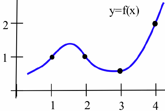
- For the function graphed below:

estimate the value of \(df\) when- \(x = 2\) and \(dx = 1\)
- \(x = 4\) and \(dx = -1\)
- \(x = 3\) and \(dx = 2\)
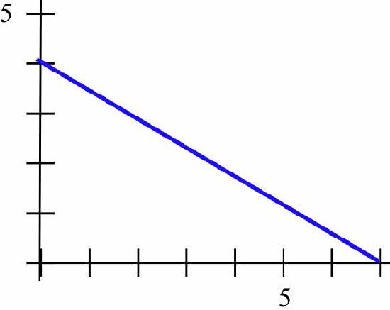
- For the function graphed below:
estimate the value of \(df\) when- \(x = 1\) and \(dx = 2\)
- \(x = 2\) and \(dx = -1\)
- \(x = 3\) and \(dx = 1\)
- Calculate the differentials \(df\) for the following functions:
- \(f(x) = x^2 - 3x\)
- \(f(x) = e^x\)
- \(f(x) = \sin( 5x )\)
- \(f(x) = x^3 + 2x\) with \(x = 1\) and \(dx = 0.2\)
- \(f(x) = \ln(x)\) with \(x = e\) and \(dx = - 0.1\)
- \(f(x) = \sqrt{2x + 5}\) with \(x = 22\) and \(dx = 3\).