4.1: Sigma Notation and Riemann Sums

One strategy for calculating the area of a region is to cut the region into simple shapes, calculate the area of each simple shape, and then add these smaller areas together to get the area of the whole region. When you use this approach with many sub-regions, it will be useful to have a notation for adding many values together: the sigma (\(\Sigma\)) notation.

summation	sigma notation	how to read it
\(1^2 + 2^2 + 3^2 + 4^2 + 5^2\)	\(\displaystyle \sum_{k=1}^{5}\, k^2\)	the sum of \(k\) squared, from \(k\) equals \(1\) to \(k\) equals \(5\)
\(\displaystyle \frac13 + \frac14 + \frac15 + \frac16 +\frac17\)	\(\displaystyle \sum_{k=3}^{7}\, \frac{1}{k}\)	the sum of \(1\) divided by \(k\), from \(k\) equals \(3\) to \(k\) equals \(7\)
\(2^0 + 2^1 + 2^2 + 2^3 + 2^4 + 2^5\)	\(\displaystyle \sum_{j=0}^{5}\, 2^j\)	the sum of \(2\) to the \(j\)-th power, from \(j\) equals \(0\) to \(j\) equals \(5\)
\(a_2 + a_3 + a_4 + a_5 + a_6 + a_7\)	\(\displaystyle \sum_{n=2}^{7}\, a_n\)	the sum of \(a\) sub \(n\), from \(n\) equals \(2\) to \(n\) equals \(7\)

The variable (typically \(i\), \(j\), \(k\), \(m\) or \(n\)) used in the summation is called the counter or index variable. The function to the right of the sigma is called the summand, while the numbers below and above the sigma are called the lower and upper limits of the summation.

Practice \(\PageIndex{1}\)

Write the summation denoted by each of the following:

1. \(\displaystyle \sum_{k=1}^{5}\, k^3\)
2. \(\displaystyle \sum_{j=2}^{7}\, \left(-1\right)^j \frac{1}{j}\)
3. \(\displaystyle \sum_{m=0}^{4}\, \left(2m+1\right)\)

Answer

1. \(\displaystyle \sum_{k=1}^{5}\, k^3 = 1 + 8 + 27 + 64 + 125\)
2. \(\displaystyle \sum_{j=2}^{7}\, \left(-1\right)^j \cdot \frac{1}{j} = \frac12 - \frac13 + \frac14 - \frac15 + \frac16 - \frac17\)
3. \(\displaystyle \sum_{m=0}^{4}\, (2m+1) = 1 + 3 + 5 + 7 + 9\)

In practice, we frequently use sigma notation together with the standard function notation: 
\begin{align*}
\sum_{k=1}^{3}\, f(k+2) &= f(1+2) + f(2+2) + f(3+2)\\
                        &= f(3) + f(4) + f(5)\\
\sum_{j=1}^{4}\, f(x_j) &= f(x_1) + f(x_2) + f(x_3) + f(x_4)
\end{align*}

Example \(\PageIndex{1}\)

Use the table:

\(x\)	\(f(x)\)	\(g(x)\)	\(h(x)\)
\(1\)	\(2\)	\(4\)	\(3\)
\(2\)	\(3\)	\(1\)	\(3\)
\(3\)	\(1\)	\(-2\)	\(3\)
\(4\)	\(0\)	\(3\)	\(3\)
\(5\)	\(3\)	\(5\)	\(3\)

to evaluate \(\displaystyle \sum_{k=2}^{5}\, 2\cdot f(k)\) and \(\displaystyle \sum_{j=3}^{5}\, \left[5+f(j-2)\right]\).

Solution

Writing out the sum and using the table values:
\begin{align*}
\sum_{k=2}^{5}\, 2\cdot f(k) &= 2\cdot f(2) + 2\cdot f(3) + 2\cdot f(4) + 2\cdot f(5)\\
                             &= 2\cdot 3 + 2\cdot 1 + 2\cdot 0 + 2\cdot 3 = 14
\end{align*}
while:
\begin{align*}
\sum_{j=3}^{5}\, \left[5+f(j-2)\right] &= \left[5+f(3-2)\right]+\left[5+f(4-2)\right]+\left[5+f(5-2)\right]\\
&= \left[5+f(1)\right]+\left[5+f(2)\right]+\left[5+f(3)\right]\\
&= \left[5+2\right]+\left[5+3\right]+\left[5+1\right]
\end{align*}
which adds up to \(21\).

Practice \(\PageIndex{2}\)

Use the values in the preceding the table from Example \(\PageIndex{1}\) to evaluate:

1. \(\displaystyle \sum_{k=2}^{5}\, g(k)\)
2. \(\displaystyle \sum_{j=1}^{4}\, h(j)\)
3. \(\displaystyle \sum_{k=3}^{5}\, \left[g(k)+f(k-1)\right]\)

Answer

1. \(\displaystyle \sum_{k=2}^{5}\, g(k) = g(2) + g(3) + g(4) + g(5) = 1 + (-2) + 3 + 5 = 7\)
2. \(\displaystyle \sum_{j=1}^{4}\, h(j) = h(1) + h(2) + h(3) + h(4) = 3 + 3 + 3 + 3 = 12\)
3. \(\displaystyle \sum_{k=3}^{5}\, \left( g(k) + f(k-1) \right) = \left(g(3) + f(2)\right) + \left(g(4) + f(3)\right) + \left(g(5) + f(4)\right) = (-2+3)+(3+1)+(5+0) = 10\)

Example \(\PageIndex{2}\)

For \(f(x) = x^2+1\), evaluate \(\displaystyle \sum_{k=0}^{3}\, f(k)\).

Solution

Writing out the sum and using the function values:
\begin{align*}
\sum_{k=0}^{3}\, f(k) &= f(0) + f(1) + f(2) + f(3)\\
                      &= \left(0^2+1\right) + \left(1^2+1\right) + \left(2^2+1\right) + \left(3^2+1\right)\\
                      &= 1+2+5+10
\end{align*}
which adds up to \(18\).

Practice \(\PageIndex{3}\)

For \(\displaystyle g(x) = \frac{1}{x}\), evaluate \(\displaystyle \sum_{k=2}^{4}\, g(k)\) and \(\displaystyle \sum_{k=1}^{3}\, g(k+1)\).

Answer

\(\displaystyle \sum_{k=2}^{4}\, g(k) = g(2) + g(3) + g(4) = \frac12 +\frac13+\frac14 =\frac{13}{12}\)

\(\displaystyle \sum_{k=1}^{3}\, g(k+1) = g(2) + g(3) + g(4) = \frac12 +\frac13+\frac14 =\frac{13}{12}\)

The summand need not contain the index variable explicitly: you can write a sum from \(k=2\) to \(k=4\) of the constant function \(f(k) = 5\) as \(\displaystyle \sum_{k=2}^{4}\, f(k)\) or \(\displaystyle \sum_{k=2}^{4}\, 5 = 5 + 5 + 5 = 3\cdot 5 = 15\). Similarly:\[\sum_{k=3}^{7}\, 2 = 2 + 2 + 2 + 2 + 2 = 5\cdot 2 = 10\nonumber\]Because the sigma notation is simply a notation for addition, it possesses all of the familiar properties of addition.

Summation Properties

Sum of Constants: \(\displaystyle \sum_{k=1}^{n}\, C = C + C + C + \cdots + C = n\cdot C\)

Addition: \(\displaystyle \sum_{k=1}^{n}\,\left(a_k + b_k\right) = \sum_{k=1}^{n}\, a_k + \sum_{k=1}^{n}\, b_k\)

Subtraction: \(\displaystyle \sum_{k=1}^{n}\,\left(a_k - b_k\right) = \sum_{k=1}^{n}\, a_k - \sum_{k=1}^{n}\, b_k\)

Constant Multiple: \(\displaystyle \sum_{k=1}^{n}\, C\cdot a_k = C\cdot  \sum_{k=1}^{n}\, a_k\)

(Problems 16 and 17 illustrate that similar patterns for sums of products and quotients are not valid.)

Sums of Areas of Rectangles

In Section 4.2, we will approximate areas under curves by building rectangles as high as the curve, calculating the area of each rectangle, and then adding the rectangular areas together.

Example \(\PageIndex{3}\)

Evaluate the sum of the rectangular areas in the figure below:

then write the sum using sigma notation. 

Solution

The sum of the rectangular areas is equal to the sum of \((\mbox{base})\cdot(\mbox{height})\) for each rectangle:\[(1)\left(\frac13\right) + (1)\left(\frac14\right) + (1)\left(\frac15\right) = \frac{47}{60}\nonumber\]which we can rewrite as \(\displaystyle \sum_{k=3}^{5}\,\frac{1}{k}\) using sigma notation.

Practice \(\PageIndex{4}\)

Evaluate the sum of the rectangular areas in the figure below:

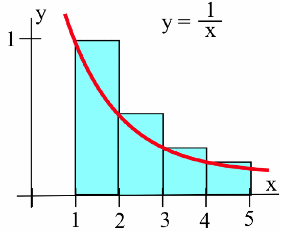
then write the sum using sigma notation.

Answer

Rectangular areas \(\displaystyle = 1 + \frac12 +\frac13+\frac14 = \frac{25}{12} = \sum_{j=1}^{4}\, \frac{1}{j}\) 

The bases of these rectangles need not be equal. For the rectangular areas associated with \(f(x)=x^2\) in the figure below:

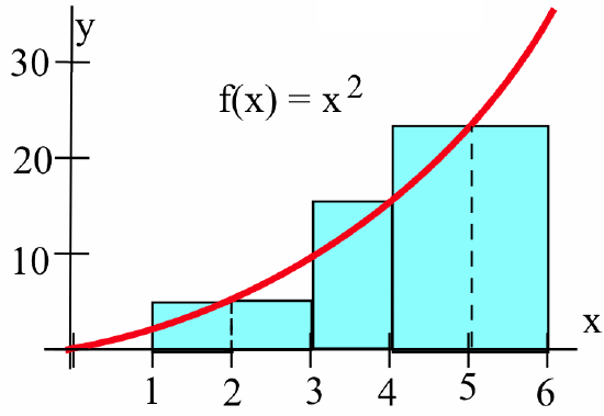
we have:

rectangle	base	height	area
\(1\)	\(3-1=2\)	\(f(2)=4\)	\(2\cdot 4 = 8\)
\(2\)	\(4-3=1\)	\(f(4)=16\)	\(1\cdot 16 = 16\)
\(3\)	\(6-4=2\)	\(f(5)=25\)	\(2\cdot 25 = 50\)

so the sum of the rectangular areas is \(8 + 16 + 50 = 74\).

Example \(\PageIndex{4}\)

Write the sum of the areas of the rectangles in the figure below:

using sigma notation. 

Solution

The area of each rectangle is \((\mbox{base})\cdot(\mbox{height})\):

rectangle	base	height	area
\(1\)	\(x_1-x_0\)	\(f(x_1)\)	\((x_1-x_0)\cdot f(x_1)\)
\(2\)	\(x_2-x_1\)	\(f(x_2)\)	\((x_2-x_1)\cdot f(x_2)\)
\(3\)	\(x_3-x_2\)	\(f(x_3)\)	\((x_3-x_2)\cdot f(x_3)\)

The area of the \(k\)-th rectangle is \(\left(x_k - x_{k-1}\right)\cdot f\left(x_k\right)\), so we can express the total area of the three rectangles as \(\displaystyle \sum_{k=1}^{3}\,\left(x_k - x_{k-1}\right)\cdot f\left(x_k\right)\).

Practice \(\PageIndex{5}\)

Write the sum of the areas of the shaded rectangles in the figure below:

using sigma notation. 

Answer

\(\displaystyle f\left(x_0\right)\cdot \left(x_1 - x_0\right) + f\left(x_1\right)\cdot \left(x_2 - x_1\right) + f\left(x_2\right)\cdot \left(x_3 - x_2\right) = \sum_{j=1}^{3}\, f\left(x_{j-1}\right)\cdot \left(x_j - x_{j-1}\right)\)

\(\displaystyle \sum_{k=0}^{2}\, f\left(x_{k}\right)\cdot \left(x_{k+1} - x_{k}\right)\) 

Area Under a Curve: Riemann Sums

Suppose we want to calculate the area between the graph of a positive function \(f\) and the \(x\)-axis on the interval \([a, b]\), as shown below left:

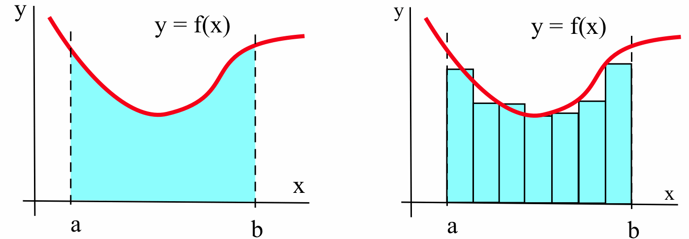
One method to approximate the area involves building several rectangles with bases on the \(x\)-axis spanning the interval \([a, b]\) and with sides that reach up to the graph of \(f\) (as shown above right). We then compute the areas of the rectangles and add them up to get a number called a Riemann sum of \(f\) on \([a, b]\). The area of the region formed by the rectangles provides an approximation of the area we want to compute.

Example \(\PageIndex{5}\)

Approximate the area shown below left between the graph of \(f\) and the \(x\)-axis spanning the interval \([2, 5]\):

by summing the areas of the rectangles shown in the figure above right.

Solution

The total area is \((2)(3) + (1)(5) = 11\) square units.

In order to effectively describe this process, some new vocabulary is helpful: a partition of an interval and the mesh of a partition.

A partition \(\cal{P}\) of a closed interval \([a,b]\) into \(n\) subintervals consists of a set of \(n+1\) points \(\left\{ x_0 = a, x_1, x_2, x_3, \ldots, x_{n-1}, x_n = b\right\}\) listed in increasing order, so that \(a= x_0 < x_1 < x_2 < x_3 < \ldots < x_{n-1} < x_n = b\). (A partition is merely a collection of points on the horizontal axis, unrelated to the function \(f\) in any way.)

The points of the partition \(\cal{P}\) divide \([a,b]\) into \(n\) subintervals:

These intervals are \([x_0, x_1]\), \([x_1, x_2]\), \([x_2, x_3]\), … , \([x_{n-1}, x_n]\) with lengths \(\Delta x_1 = x_1 - x_0\), \(\Delta x_2 = x_2 - x_1\), \(\Delta x_3 = x_3 - x_2, … , \Delta x_n = x_n - x_{n-1}\). The points \(x_k\) of the partition \(\cal{P}\) mark the locations of the vertical lines for the sides of the rectangles, and the bases of the rectangles have lengths \(\Delta x_k\) for \(k = 1\), \(2\), \(3\), … , \(n\). The mesh or norm of a partition \(\cal{P}\) is the length of the longest of the subintervals \([x_{k-1}, x_k]\) or, equivalently, the maximum value of \(\Delta x_k\) for \(k = 1\), \(2\), \(3\), … , \(n\).

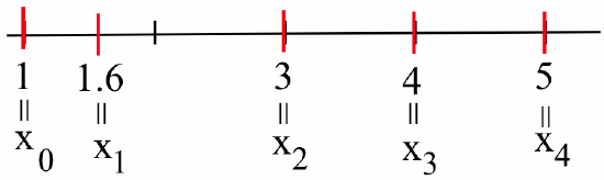
For example, the set \({\cal P} = \left\{2, 3, 4.6, 5.1, 6\right\}\) is a partition of the interval \([2,6]\):

that divides the interval \([2,6]\) into four subintervals with lengths \(\Delta x_1 = 1\), \(\Delta x_2 = 1.6\), \(\Delta x_3 = 0.5\) and \(\Delta x_4 = 0.9\), so the mesh of this partition is \(1.6\), the maximum of the lengths of the subintervals. (If the mesh of a partition is “small,” then the length of each one of the subintervals is the same or smaller.)

Practice \(\PageIndex{6}\)

\({\cal P} = \{3, 3.8, 4.8, 5.3, 6.5, 7, 8\}\) is a partition of what interval? How many subintervals does it create? What is the mesh of the partition? What are the values of \(x_2\) and \(\Delta x_2\)?

Answer

Interval is \([3, 8]\); six subintervals; mesh \(= 1.2\); \(x_2 = 4.8\); \(\Delta x_2 = x_2 - x_1 = 4.8 - 3.8 = 1\). 

A function, a partition and a point chosen from each subinterval determine a Riemann sum. Suppose \(f\) is a positive function on the interval \([a,b]\) (so that \(f(x) > 0\) when \(a \leq x \leq b\)), \({\cal P} = \left\{ x_0 = a, x_1, x_2, x_3, \ldots, x_{n-1}, x_n = b\right\}\) is a partition of \([a,b]\), and \(c_k\) is an \(x\)-value chosen from the \(k\)-th subinterval \([x_{k-1}, x_k]\) (so \(x_{k-1} \leq c_k \leq x_k\)). Then the area of the \(k\)-th rectangle is:\[f\left(c_k\right)\cdot\left(x_k - x_{k-1}\right) = f\left(c_k\right)\cdot\Delta x_k\nonumber\]

Definition

A summation of the form \(\displaystyle \sum_{k=1}^{n}\, f\left(c_k\right)\cdot\Delta x_k\) is called a Riemann sum of \(f\) for the partition \(\cal{P}\) and the chosen points \(\left\{c_1, c_2,\ldots, c_n\right\}\).

This Riemann sum is the total of the areas of the rectangular regions and provides an approximation of the area between the graph of \(f\) and the \(x\)-axis on the interval \([a,b]\).

Example \(\PageIndex{6}\)

Find the Riemann sum for \(\displaystyle f(x) = \frac{1}{x}\) using the partition \(\{1, 4, 5\}\) and the values \(c_1 = 2\) and \(c_2 = 5\):

Solution

The two subintervals are \([1,4]\) and \([4,5]\), hence \(\Delta x_1 = 3\) and \(\Delta x_2 = 1\). So the Riemann sum for this partition is: 
\begin{align*} \sum_{k=1}^{2}\, f\left(c_k\right)\cdot\Delta x_k &= f\left(c_1\right)\cdot\Delta x_1 + f\left(c_2\right)\cdot\Delta x_2\\
&= f(2)\cdot 3 + f(5)\cdot 1  = \frac12 \cdot 3 + \frac15 \cdot 1 = \frac{17}{10}\end{align*} 
The value of the Riemann sum is \(1.7\).

Practice \(\PageIndex{7}\)

Calculate the Riemann sum for \(\displaystyle f(x) = \frac{1}{x}\) on the partition \(\{1, 4, 5\}\) using the chosen values \(c_1 = 3\) and \(c_2 = 4\).

Answer

RS \(= (3)\left(\frac13\right) + (1)\left(\frac14\right) = 1.25\)

Practice \(\PageIndex{8}\)

What is the smallest value a Riemann sum for \(\displaystyle f(x) = \frac{1}{x}\) can have using the partition \(\{1, 4, 5\}\)? (You will need to choose values for \(c_1\) and \(c_2\).) What is the largest value a Riemann sum can have for this function and partition?

Answer

smallest RS \(= (3)\left(\frac14\right) + (1)\left(\frac15\right) = 0.95\) BREAK largest RS \(= (3)( 1 ) + (1)\left(\frac14\right) = 3.25\)

The table below shows the output of a computer program that calculated Riemann sums for the function \(\displaystyle f(x) = \frac{1}{x}\) with various numbers of subintervals (denoted \(n\)) and different ways of choosing the points \(c_k\) in each subinterval.

\(n\)	mesh	\(c_k = \text{left edge} = x_{k-1}\)	\(c_k = \text{"random" point}\)	\(c_k = \text{right edge} = x_k\)
\(4\)	\(1.0\)	\(2.083333\)	\(1.473523\)	\(1.283333\)
\(8\)	\(0.5\)	\(1.828968\)	\(1.633204\)	\(1.428968\)
\(16\)	\(0.25\)	\(1.714406\)	\(1.577806\)	\(1.514406\)
\(40\)	\(0.10\)	\(1.650237\)	\(1.606364\)	\(1.570237\)
\(400\)	\(0.01\)	\(1.613446\)	\(1.609221\)	\(1.605446\)
\(4000\)	\(0.001\)	\(1.609838\)	\(1.609436\)	\(1.609038\)

(As the mesh gets smaller, all of the Riemann Sums seem to be approaching the same value, approximately \(1.609\). As we shall soon see, these values are all approaching \(\ln(5) \approx 1.609437912\).)
 
When the mesh of the partition is small (and the number of subintervals, \(n\), is large), it appears that all of the ways of choosing the \(c_k\) locations result in approximately the same value for the Riemann sum. For this decreasing function, using the left endpoint of the subinterval always resulted in a sum that was larger than the area approximated by the sum. Choosing the right endpoint resulted in a value smaller than that area. Why? 

Example \(\PageIndex{7}\)

Find the Riemann sum for the function \(f(x) = \sin(x)\) on the interval \([0, \pi]\) using the partition \(\displaystyle \left\{0, \frac{\pi}{4}, \frac{\pi}{2}, \pi\right\}\) and the chosen points \(\displaystyle c_1 = \frac{\pi}{4}\), \(\displaystyle c_2 = \frac{\pi}{2}\) and \(\displaystyle c_3 = \frac{3\pi}{4}\).

Solution

The three subintervals are \(\displaystyle \left[0, \frac{\pi}{4}\right]\), \(\displaystyle \left[\frac{\pi}{4}, \frac{\pi}{2}\right]\) and \(\displaystyle \left[\frac{\pi}{2}, \pi\right]\):

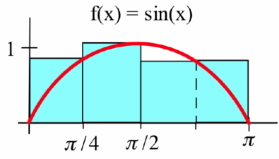
so \(\Delta x_1 = \frac{\pi}{4}\), \(\Delta x_2 = \frac{\pi}{4}\) and \(\Delta x_3 = \frac{\pi}{2}\). The Riemann sum for this partition is:
\begin{align*} \sum_{k=1}^{3}\, f\left(c_k\right)\cdot\Delta x_k &= \sin\left(\frac{\pi}{4}\right)\cdot \frac{\pi}{4} + \sin\left(\frac{\pi}{2}\right)\cdot \frac{\pi}{4} + \sin\left(\frac{3\pi}{4}\right)\cdot \frac{\pi}{2}\\
&= \frac{\sqrt{2}}{2} \cdot \frac{\pi}{4} + 1\cdot \frac{\pi}{4} + \frac{\sqrt{2}}{2} \cdot \frac{\pi}{2} = \frac{(2+3\sqrt{2})\pi}{8}\end{align*}
or approximately \(2.45148\).

Practice \(\PageIndex{9}\)

Find the Riemann sum for the function and partition in the previous Example, but this time choose \(c_1 = 0\), \(\displaystyle c_2 = \frac{\pi}{2}\) and \(\displaystyle c_3 = \frac{\pi}{2}\).

Answer

RS \(= (0)\left(\frac{\pi}{4}\right) + (1)\left(\frac{\pi}{4}\right) + (1)\left(\frac{\pi}{2}\right) \approx 2.356\)

Two Special Riemann Sums: Lower and Upper Sums

Two particular Riemann sums are of special interest because they represent the extreme possibilities for a given partition.

Note

We need \(f\) to be continuous in order to assure that it attains its minimum and maximum values on any closed subinterval of the partition. If \(f\) is bounded — but not necessarily continuous — we can generalize this definition by replacing \(f\left(m_k\right)\) with the greatest lower bound of all \(f(x)\) on the interval and \(f\left(M_k\right)\) with the least upper bound of all \(f(x)\) on the interval.

Definition

If \(f\) is a positive, continuous function on \([a,b]\) and \(\cal{P}\) is a partition of \([a,b]\), let \(m_k\) be the \(x\)-value in the \(k\)-th subinterval so that \(f\left(m_k\right)\) is the minimum value of \(f\) on that interval,  and let \(M_k\) be the \(x\)-value in the \(k\)-th subinterval so that \(f\left(M_k\right)\) is the maximum value of \(f\) on that subinterval. Then:

\(\displaystyle \mbox{LS}_{\cal P} = \sum_{k=1}^{n}\, f\left(m_k\right)\cdot\Delta x_k\) is the lower sum of \(f\) for \(\cal{P}\)

\(\displaystyle \mbox{US}_{\cal P} = \sum_{k=1}^{n}\, f\left(M_k\right)\cdot\Delta x_k\) is the upper sum of \(f\) for \(\cal{P}\)

 

Geometrically, a lower sum arises from building rectangles under the graph of \(f\):

and every lower sum is less than or equal to the exact area \(A\) of the region bounded by the graph of \(f\)  and the \(x\)-axis on the interval \([a,b]\): \(\displaystyle \mbox{LS}_{\cal P} \leq A\) for every partition \(\cal{P}\).

Likewise, an upper sum arises from building rectangles over the graph of \(f\):

and every upper sum is greater than or equal to the exact area \(A\) of the region bounded by the graph of \(f\) and the \(x\)-axis on the interval \([a,b]\): \(\displaystyle \mbox{US}_{\cal P} \geq A\) for every partition \({\cal P}\). 

Together, the lower and upper sums provide bounds on the size of the exact area: \(\displaystyle \mbox{LS}_{\cal P} \leq A \leq \mbox{US}_{\cal P}\).

For any \(c_k\) value in the \(k\)-th subinterval, \(f\left(m_k\right) \leq f\left(c_k\right) \leq f\left(M_k\right)\), so, for any choice of the \(c_k\) values, the Riemann sum \(\displaystyle \mbox{RS}_{\cal P} = \sum_{k=1}^{n}\, f\left(c_k\right)\cdot\Delta x_k\) satisfies the inequality:\[\sum_{k=1}^{n}\, f\left(m_k\right)\cdot\Delta x_k \quad \leq \quad \sum_{k=1}^{n}\, f\left(c_k\right)\cdot\Delta x_k \quad \leq \quad \sum_{k=1}^{n}\, f\left(M_k\right)\cdot\Delta x_k\nonumber\]or, equivalently, \(\displaystyle \mbox{LS}_{\cal P} \leq \mbox{RS}_{\cal P} \leq \mbox{US}_{\cal P}\). The lower and upper sums provide bounds on the size of all Riemann sums for a given partition.

The exact area \(A\) and every Riemann sum \(\displaystyle \mbox{RS}_{\cal P}\) for partition \(\cal{P}\) and any choice of points \(\left\{c_k\right\}\) both lie between the lower sum and the upper sum for \(\cal{P}\):

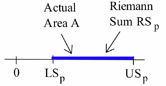
Therefore, if the lower and upper sums are close together, then the area and any Riemann sum for \(\cal{P}\) (regardless of how you choose the points \(c_k\)) must also be close together. If we know that the upper and lower sums for a partition \(\cal{P}\) are within \(0.001\) units of each other, then we can be sure that every Riemann sum for partition \(\cal{P}\) is within \(0.001\) units of the exact area \(A\).

Unfortunately, finding minimums and maximums for each subinterval of a partition can be a time-consuming (and tedious) task, so it is usually not practical to determine lower and upper sums for “wiggly” functions. If \(f\) is monotonic, however, then it is easy to find the values for \(m_k\) and \(M_k\), and sometimes we can even explicitly calculate the limits of the lower and upper sums.

For a monotonic, bounded function we can guarantee that a Riemann sum is within a certain distance of the exact value of the area it is approximating. 

(Recall from Section 3.3 that “monotonic” means “always increasing or always decreasing” on the interval in question.)

Theorem

If: \(f\) is a positive, monotonic, bounded function on \([a,b]\)

then: for any partition \(\cal{P}\) and any Riemann sum for \(f\) using \(\cal{P}\),\[\left|\mbox{RS}_{\cal P}-A\right| \leq \mbox{US}_{\cal P}-\mbox{LS}_{\cal P} \leq \left|f(b) - f(a)\right|\cdot \left(\mbox{mesh of }{\cal P}\right)\nonumber\]

(In words, this string of inequalities says that the distance between any Riemann sum and the area being approximated is no bigger than the difference between the upper and lower Riemann sums for the same partition, which in turn is no bigger than the distance between the values of the function at the endpoints of the interval times the mesh of the partition.)

Proof

The Riemann sum and the exact area are both between the upper and lower sums, so the distance between the Riemann sum and the exact area is no bigger than the distance between the upper  and lower sums. If \(f\) is monotonically increasing, we can slide the areas representing the difference of the upper and lower sums into a rectangle:

whose height equals \(f(b)-f(a)\) and whose base equals the mesh of \(\cal{P}\). So the total difference of the upper and lower sums is smaller than the area of that rectangle, \(\displaystyle \left[f(b) - f(a)\right]\cdot \left(\mbox{mesh of }{\cal P}\right)\).

(See Problem 56 for the monotonically decreasing case.)

Problems

In Problems 1–6 , rewrite the sigma notation as a summation and perform the indicated addition.

1. \(\displaystyle \sum_{k=2}^{4}\, k^2\)
2. \(\displaystyle \sum_{j=1}^{5}\, (1 + j)\)
3. \(\displaystyle \sum_{n=1}^{3}\, (1 + n)^2\)
4. \(\displaystyle \sum_{k=0}^{5}\, \sin(\pi k)\)
5. \(\displaystyle \sum_{j=0}^{5}\, \cos(\pi j)\)
6. \(\displaystyle \sum_{k=1}^{3}\, \frac{1}{k}\)

In Problems 7–12, rewrite each summation using the sigma notation. Do not evaluate the sums.

7. \(3 + 4 + 5 + \cdots + 93 + 94\)
8. \(4 + 6 + 8 + \cdots + 24\)
9. \(9 + 16 + 25 + 36 + \cdots + 144\)
10. \(\displaystyle \frac34 + \frac39 + \frac{3}{16} + \cdots + \frac{3}{100}\)
11. \(1\cdot 2^1 + 2\cdot 2^2 + 3\cdot 2^3 + \cdots + 7\cdot 2^7\)
12. \(3 + 6 + 9 + \cdots + 30\)

In Problems 13--15, use this table:

\(k\)	\(a_k\)	\(b_k\)
\(1\)	\(1\)	\(2\)
\(2\)	\(2\)	\(2\)
\(3\)	\(3\)	\(2\)

to verify the equality for these values of \(a_k\) and \(b_k\).

13. \(\displaystyle \sum_{k=1}^{3}\, \left(a_k + b_k\right) = \sum_{k=1}^{3}\, a_k + \sum_{k=1}^{3}\, b_k\)
14. \(\displaystyle \sum_{k=1}^{3}\, \left(a_k - b_k\right) = \sum_{k=1}^{3}\, a_k - \sum_{k=1}^{3}\, b_k\)
15. \(\displaystyle \sum_{k=1}^{3}\, 5 a_k = 5\cdot \sum_{k=1}^{3}\, a_k\)

For Problems 16–18, use the values of \(a_k\) and \(b_k\) in the table above to verify the inequality.

16. \(\displaystyle \sum_{k=1}^{3}\, a_k \cdot b_k \neq \left(\sum_{k=1}^{3}\, a_k\right) \left(\sum_{k=1}^{3}\, b_k\right)\)
17. \(\displaystyle \sum_{k=1}^{3}\, a_k^2 \neq \left(\sum_{k=1}^{3}\, a_k\right)^2\)
18. \(\displaystyle \sum_{k=1}^{3}\, \frac{a_k}{b_k} \neq \frac{\sum_{k=1}^{3}\, a_k}{\sum_{k=1}^{3}\, b_k}\)

For Problems 19–30, \(f(x) = x^2\), \(g(x) = 3x\) and \(\displaystyle h(x) = \frac{2}{x}\). Evaluate each sum.

19. \(\displaystyle \sum_{k=0}^{3}\, f(k)\)
20. \(\displaystyle \sum_{k=0}^{3}\, f(2k)\)
21. \(\displaystyle \sum_{j=0}^{3}\, 2\cdot f(j)\)
22. \(\displaystyle \sum_{i=0}^{3}\, f(1+i)\)
23. \(\displaystyle \sum_{m=1}^{3}\, g(m)\)
24. \(\displaystyle \sum_{k=1}^{3}\, g\left(f(k)\right)\)
25. \(\displaystyle \sum_{j=1}^{3}\, g^2(j)\)
26. \(\displaystyle \sum_{k=1}^{3}\, k\cdot g(k)\)
27. \(\displaystyle \sum_{k=2}^{4}\, h(k)\)
28. \(\displaystyle \sum_{i=1}^{4}\, h(3i)\)
29. \(\displaystyle \sum_{n=1}^{3}\, f(n)\cdot h(n)\)
30. \(\displaystyle \sum_{k=1}^{7}\, g(k)\cdot h(k)\)

In Problems 31–36, write out each summation and simplify the result. These are examples of “telescoping sums.”

31. \(\displaystyle \sum_{k=1}^{7}\, \left[k^2-(k-1)^2\right]\)
32. \(\displaystyle \sum_{k=1}^{6}\, \left[k^3-(k-1)^3\right]\)
33. \(\displaystyle \sum_{k=1}^{5}\, \left[\frac{1}{k}-\frac{1}{k+1}\right]\)
34. \(\displaystyle \sum_{k=0}^{4}\, \left[(k+1)^3-k^3\right]\)
35. \(\displaystyle \sum_{k=0}^{8}\, \left[\sqrt{k+1}-\sqrt{k}\right]\)
36. \(\displaystyle \sum_{k=1}^{5}\, \left[x_k-x_{k-1}\right]\)

In Problems 37–43:

1. list the subintervals determined by the partition \(\cal{P}\)
2. find the values of \(\Delta x_k\),
3. find the mesh of \(\cal{P}\) and (d) calculate \(\displaystyle \sum_{k=1}^{n}\, \Delta x_k\).

37. \({\cal P} = \{2, 3, 4.5, 6, 7\}\)
38. \({\cal P} = \{3, 3.6, 4, 4.2, 5, 5.5, 6\}\)
39. \({\cal P} = \{-3, -1, 0, 1.5, 2\}\)
40. \({\cal P}\) as shown below:
    
41. \({\cal P}\) as shown below:
    
42. \({\cal P}\) as shown below:
    
43. For \(\Delta x_k = x_k - x_{k-1}\), verify that:\[\sum_{k=1}^{n}\, \Delta x_k = \mbox{length of the interval } [a, b]\nonumber\]

For Problems 44–48, sketch a graph of \(f\), draw vertical lines at each point of the partition, evaluate each \(f\left(c_k\right)\) and sketch the corresponding rectangle, and calculate and add up the areas of those rectangles.

44. \(f(x) = x + 1\), \({\cal P} = \{1, 2, 3, 4\}\)
    1. \(c_1 = 1\), \(c_2 = 3\), \(c_3 = 3\)
    2. \(c_1 = 2\), \(c_2 = 2\), \(c_3 = 4\)
45. \(f(x) = 4 - x^2\), \({\cal P} = \{0, 1, 1.5, 2\}\)
    1. \(c_1 = 0\), \(c_2 = 1\), \(c_3 = 2\)
    2. \(c_1 = 1\), \(c_2 = 1.5\), \(c_3 = 1.5\)
46. \(f(x) = \sqrt{x}\), \({\cal P} = \{0, 2, 5, 10\}\)
    1. \(c_1 = 1\), \(c_2 = 4\), \(c_3 = 9\)
    2. \(c_1 = 0\), \(c_2 = 3\), \(c_3 = 7\)
47. \(f(x) = \sin(x)\), \({\cal P} = \left\{0, \frac{\pi}{4}, \frac{\pi}{2}, \pi\right\}\)
    1. \(c_1 = 0\), \(\displaystyle c_2 = \frac{\pi}{4}\), \(\displaystyle c_3 = \frac{\pi}{2}\)
    2. \(\displaystyle c_1 = \frac{\pi}{4}\), \(\displaystyle c_2 = \frac{\pi}{2}\), \(c_3 = \pi\)
48. \(f(x) = 2^x\), \({\cal P} = \{0, 1, 3\}\)
    1. \(c_1 = 0\), \(c_2 = 2\)
    2. \(c_1 = 1\), \(c_2 = 3\)

For Problems 49–52, sketch the function and find the smallest possible value and the largest possible value for a Riemann sum for the given function and partition.

49. \(f(x) = 1 + x^2\)
    1. \({\cal P} = \{1, 2, 4, 5\}\)
    2. \({\cal P} = \{1, 2, 3, 4, 5\}\)
    3. \({\cal P} = \{1, 1.5, 2, 3, 4, 5\}\)
50. \(f(x) = 7 - 2x\)
    1. \({\cal P} = \{0, 2, 3\}\)
    2. \({\cal P} = \{0, 1, 2, 3\}\)
    3. \({\cal P} = \{0, .5, 1, 1.5, 2, 3\}\)
51. \(f(x) = \sin(x)\)
    1. \({\cal P} = \left\{0, \frac{\pi}{2}, \pi\right\}\)
    2. \({\cal P} = \left\{0, \frac{\pi}{4}, \frac{\pi}{2}, \pi \right\}\)
    3. \({\cal P} = \left\{0, \frac{\pi}{4}, \frac{3\pi}{4}, \pi\right\}\)
52. \(f(x) = x^2 - 2x + 3\)
    1. \({\cal P} = \{0, 2, 3\}\)
    2. \({\cal P} = \{0, 1, 2, 3\}\)
    3. \({\cal P} = \{0, 0.5, 1, 2, 2.5, 3\}\)
53. Suppose \(\displaystyle \mbox{LS}_{\cal{P}} = 7.362\) and \(\displaystyle \mbox{US}_{\cal{P}} = 7.402\) for a positive function \(f\) and a partition \(\cal{P}\) of \([1, 5]\).
    1. You can be certain that every Riemann sum for the partition \(\cal{P}\) is within what distance of the exact value of the area between the graph of \(f\) and the \(x\)-axis on the interval \([1, 5]\)?
    2. What if \(\displaystyle \mbox{LS}_{\cal{P}} = 7.372\) and \(\displaystyle \mbox{US}_{\cal{P}} = 7.390\)?
54. Suppose you divide the interval \([1, 4]\) into \(100\) equally wide subintervals and calculate a Riemann sum for \(f(x) = 1 + x^2\) by randomly selecting a point \(c_k\) in each subinterval.
    1. You can be certain that the value of the Riemann sum is within what distance of the exact value of the area between the graph of \(f\) and the \(x\)-axis on interval \([1, 4]\)?
    2. What if you use \(200\) equally wide subintervals?
55. If you divide \([2, 4]\) into \(50\) equally wide subintervals and calculate a Riemann sum for \(f(x) = 1 + x^3\) by randomly selecting a point \(c_k\) in each subinterval, then you can be certain that the Riemann sum is within what distance of the exact value of the area between \(f\) and the \(x\)-axis on the interval \([2, 4]\)?
56. If \(f\) is monotonic decreasing on \([a, b]\) and you divide \([a, b]\) into \(n\) equally wide subintervals:
    
    then you can be certain that the Riemann sum is within what distance of the exact value of the area between \(f\) and the \(x\)-axis on the interval \([a, b]\)?

Summing Powers of Consecutive Integers

Formulas for some commonly encountered summations can be useful for explicitly evaluating certain special Riemann sums. (The formulas below are included here for your reference.  They will not be used in the following sections, except for a handful of exercises in Section 4.2.)

The summation formula for the first \(n\) positive integers is relatively well known, has several easy but clever proofs, and even has an interesting story behind it.\[1 + 2 + 3 + \cdots + (n-1) + n = \sum_{k=1}^{n}\, k = \frac{n(n+1)}{2}\nonumber\]

Proof

Let \(S = 1 + 2 + 3 + \cdots + (n-2) + (n-1) + n\), which we can also write as \(S = n + (n-1) + (n-2) + \cdots + 3 + 2 + 1\). Adding these two representations of \(S\) together:

\(S =\)

\(1\)

\(+\)

\(2\)

\(+\)

\(3\)

\(+\)

\(\cdots\)

\(+\)

\((n-2)\)

\(+\)

\((n-1)\)

\(+\)

\(n\)

\(+\ S =\)

\(n\)

\(+\)

\((n-1)\)

\(+\)

\((n-2)\)

\(+\)

\(\cdots\)

\(+\)

\(3\)

\(+\)

\(2\)

\(+\)

\(1\)

\(2S =\)

\((n+1)\)

\(+\)

\((n+1)\)

\(+\)

\((n+1)\)

\(+\)

\(\cdots\)

\(+\)

\((n+1)\)

\(+\)

\((n+1)\)

\(+\)

\((n+1)\)

So \(\displaystyle 2S = n\cdot(n+1) \Rightarrow S = \frac{n(n+1)}{2}\), the desired formula.

Note

Karl Friedrich Gauss (1777–1855), a German mathematician sometimes called the “prince of mathematics,” supposedly discovered this formula for himself at the age of five when his teacher, planning to keep the class busy for a while, asked the students to add up the integers from 1 to 100. Gauss thought a few minutes, wrote his answer on his slate, and turned it in, then sat smugly while his classmates struggled with the problem.

57. Find the sum of the first 100 positive integers in two ways:
    1. using Gauss’ formula, and
    2. using Gauss’ method (from the proof).
58. Find the sum of the first 10 odd integers. (Each odd integer can be written in the form \(2k - 1\) for \(k = 1\), \(2\), \(3\), … .)
59. Find the sum of the integers from \(10\) to \(20\).

Formulas for other integer powers of the first \(n\) integers are also known:

\begin{align*} \sum_{k=1}^{n}\, k &=& \frac12 n^2 + \frac12 n &= \frac{n(n+1)}{2}\\ \sum_{k=1}^{n}\, k^2 &=& \frac13 n^3 + \frac12 n^2 + \frac16 n &= \frac{n(n+1)(2n+1)}{6}\\ \sum_{k=1}^{n}\, k^3 &=& \frac14 n^ 4 + \frac12 n^3 + \frac14 n^2 &= \left(\frac{n(n+1)}{2}\right)^2\\ \sum_{k=1}^{n}\, k^4 &=& \frac15 n^5 + \frac12 n^ 4 + \frac13 n^3 - \frac{1}{30}n &= \frac{n(n+1)(2n+1)(3n^2+3n-1)}{30} \end{align*}

In Problems 60–62, use the properties of summation and the formulas for powers given above to evaluate each sum.

60. \(\displaystyle \sum_{k=1}^{10}\, \left(3 + 2k + k^2\right)\)
61. \(\displaystyle \sum_{k=1}^{10}\, k\cdot \left(k^2+1\right)\)
62. \(\displaystyle \sum_{k=1}^{10}\, k^2\cdot \left(k-3\right)\)