4.2: The Definite Integral

Each particular Riemann sum depends on several things: the function \(f\), the interval \([a,b]\), the partition \({\cal P}\) of that interval, and the chosen values \(c_k\) from each subinterval of that partition. Fortunately — for most of the functions needed for applications — as the approximating rectangles get thinner (and as the meshes of the partitions \({\cal P}\) approach \(0\) and  the number of subintervals \(n\) in those partitions approaches \(\infty\)) the values of the Riemann sums approach the same number, independent of the particular partitions \(P\) and the chosen points \(c_k\) in the subintervals of those partitions.

This limit of the Riemann sums will become the next big topic in calculus: the definite integral. Integrals arise throughout the rest of this book and in applications in almost every field that uses mathematics.

Definition of the Definite Integral

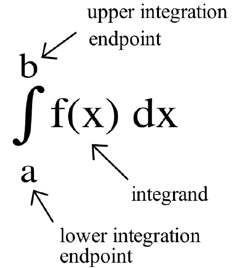
If \(\displaystyle \lim_{\left\|{\cal P}\right\| \to 0}\, \left( \sum_{k=1}^{n}\, f\left(c_k\right)\cdot\Delta x_k\right)\) equals a finite number \(I\), where each \({\cal P}\) is a partition of the interval \([a, b]\), then we say a bounded function \(f\) is integrable on the interval \([a, b]\) and call the number \(I\) the definite integral of \(f\) on \([a,b]\) and write it as \(\displaystyle \int_a^b f(x)\, dx\).

Note

Here we use the notation \(\left\|{\cal P}\right\|\) to mean “the mesh of \({\cal P}\)” and we assume \(b>a\) so that \([a,b]\) is not a single point.

The \(dx\) is a differential (see Section 3.6), the limit of the discrete quantity \(\Delta x\) in the Riemann sum.

We read the symbol \(\displaystyle \int_a^b f(x)\, dx\)  as “the integral from \(a\) to \(b\) of ‘eff’ of \(x\) ‘dee’ \(x\)” or “the integral from \(a\) to \(b\) of \(f(x)\) with respect to \(x\).”  Furthermore, we call \(f(x)\) the integrand, \(a\) the lower endpoint of integration and \(b\) the upper endpoint of integration. (We will sometimes also call \(a\) and \(b\) the upper and lower limits of integration.)

Example \(\PageIndex{1}\)

Describe the area between the graph of \(\displaystyle f(x) = \frac{1}{x}\), the \(x\)-axis, and the vertical lines at \(x = 1\) and \(x = 5\) as a limit of Riemann sums and as a definite integral.

Solution

Here \(\displaystyle f(x) = \frac{1}{x}\), \(a = 1\) and \(b=5\), so:\[\mbox{area} =  \lim_{\left\|{\cal P}\right\| \to 0}\, \left( \sum_{k=1}^{n}\, \frac{1}{c_k}\cdot\Delta x_k\right) = \int_1^5 \frac{1}{x}\, dx\nonumber\]which, according to estimations made in Section 4.1, is approximately equal to \(1.609\).

Note

You may have noticed that we did not precisely define what \(\displaystyle \lim_{\left\|{\cal P}\right\| \to 0}\) means or how to compute this limit. Providing a definition turns out to be more complicated than the limits we have encountered so far, and in practice we will rarely need to compute such a limit, so a formal definition is left to more advanced textbooks.

Practice \(\PageIndex{1}\)

Describe the area between the graph of \(f(x)= \sin(x)\), the \(x\)-axis, and the vertical lines at \(x = 0\) and \(x = \pi\) as a limit of Riemann sums and as a definite integral.

Answer

area \(\displaystyle = \lim_{\left\|{\cal P}\right\| \to 0}\, \left( \sum_{k=1}^{n}\, \sin\left(c_k\right)\cdot\Delta x_k\right) = \int_0^{\pi}\sin(x)\, dx\)

Example \(\PageIndex{2}\)

Using the concept of area, determine the values of:

1. \(\displaystyle \lim_{\left\|{\cal P}\right\| \to 0}\, \left( \sum_{k=1}^{n}\, \left(1+c_k\right)\cdot\Delta x_k\right)\) on the interval \([1,3]\)
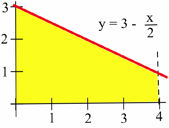
2. \(\displaystyle \int_0^4 \left(5-x\right)\, dx\)
3. \(\displaystyle \int_{-1}^1 \sqrt{1-x^2}\, dx\)

Solution

1. The limit of the Riemann sums represents the area between the graph of \(f(x) = 1+x\), the \(x\)-axis, and the vertical lines at \(x=1\) and \(x=3\):
   
   This area equals \(6\) square units.
2. The definite integral represents the area between \(f(x) = 5 - x\), the \(x\)-axis and the vertical lines at \(x=0\) and \(x=4\), which is a trapezoid with area \(12\) square units.
3. The definite integral represents the area of the upper half of the circle \(x^2 + y^2 = 1\), which has radius \(1\) and center at \((0,0)\). The area of this semicircle is \(\displaystyle \frac12 \cdot \pi r^2 = \frac12 \cdot \pi \cdot 1^2 = \frac{\pi}{2}\).

Practice \(\PageIndex{2}\)

Using the concept of area, determine the values of:

1. \(\displaystyle \lim_{\left\|{\cal P}\right\| \to 0}\, \left( \sum_{k=1}^{n}\, \left(2c_k\right)\cdot\Delta x_k\right)\) on the interval \([1,3]\)
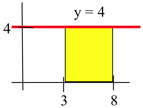
2. \(\displaystyle \int_3^8 4\, dx\)

Answer

\(\displaystyle \lim_{\left\|{\cal P}\right\| \to 0}\, \left( \sum_{k=1}^{n}\, \left(2c_k\right)\cdot\Delta x_k\right) =\) area of trapezoid in the figure below \(=8\)

\(\displaystyle \int_3^8 4\, dx =\) area of rectangle in figure below \(= 20\)

Example \(\PageIndex{3}\)

Represent each limit of Riemann sums as a definite integral.

1. \(\displaystyle \lim_{\left\|{\cal P}\right\| \to 0}\, \left( \sum_{k=1}^{n}\, \left(3+c_k\right) \Delta x_k\right)\) on \([1,4]\)
2. \(\displaystyle \lim_{\left\|{\cal P}\right\| \to 0}\, \left( \sum_{k=1}^{n}\, \sqrt{c_k} \, \Delta x_k\right)\) on \([0,9]\)

Solution

1. \(\displaystyle \int_1^4 \left(3+x\right)\, dx\)
2. \(\displaystyle \int_0^9 \sqrt{x}\, dx\)

Example \(\PageIndex{4}\)

Represent each shaded area in the figure below as a definite integral:

(Do not attempt to evaluate the definite integral, just translate the picture into symbols.)

Solution

1. \(\displaystyle \int_{-2}^2 \left(4-x^2\right)\, dx\)
2. \(\displaystyle \int_0^{\pi} \sin(x)\, dx\)

The value of a definite integral \(\displaystyle \int_a^b f(x)\, dx\) depends only on the function \(f\) being integrated and on the interval \([a, b]\). Replacing the variable \(x\) that appears in \(\displaystyle \int_a^b f(x)\, dx\), sometimes called a “dummy variable,” does not change the value of the integral. The following definite integrals each represent the integral of the function \(f\) on the interval \([a,b]\), and they are all equal:\[\int_a^b f(x)\, dx \quad = \quad \int_a^b f(t)\, dt \quad = \quad \int_a^b f(u)\, du \quad = \quad \int_a^b f(w)\, dw\nonumber\]

Definite Integrals of Negative Functions

A definite integral is a limit of Riemann sums, and you can form Riemann sums using any integrand function \(f\), positive or negative (or both), continuous or discontinuous. The definite integral of an integrable function will still have a geometric meaning even if the function is sometimes (or always) negative, and definite integrals of negative functions also have meaningful interpretations in applications.

Example \(\PageIndex{5}\)

Find the definite integral of \(f(x) = -2\) on \([1,4]\). 

Solution

Writing a Riemann sum for \(f(x) = -2\) on the interval \([1,4]\):\[\sum_{k=1}^n \, f\left(c_k\right)\cdot\Delta x_k = \sum_{k=1}^n \, \left(-2\right)\cdot\Delta x_k = -2\cdot \sum_{k=1}^n \,\Delta x_k = -2\left(3\right) = -6\nonumber\]for every partition \({\cal P}\) and every choice of values for \(c_k\) so:\[\int_1^4 -2\, dx =  \lim_{\left\|{\cal P}\right\| \to 0}\, \left( \sum_{k=1}^{n}\, (-2)\cdot\Delta x_k\right) = \lim_{\left\|{\cal P}\right\| \to 0}\, -6 = -6\nonumber\]The area of the region in the figure below is \(6\) units:

but because the region is below the \(x\)-axis, the value of the integral is \(-6\).

If the graph of \(f(x)\) is below the \(x\)-axis for \(a \leq x \leq b\) (\(f\) is negative) then \(\displaystyle \int_a^b f(x)\, dx\) is \(-1\) times the area of the region below the \(x\)-axis and above the graph of \(f(x)\) between \(x=a\) and \(x=b\).

If \(f(t)\) represents the rate of population change (people per year) for a town, then negative values of \(f\) for a given time interval would indicate that the population of the town was getting smaller, and the definite integral (now a negative number) would represent the change in the population — a decrease — during that time interval.

Example \(\PageIndex{6}\)

In 1980 there were 12,000 ducks nesting around a lake. The rate of population change is shown below:

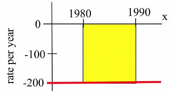
Write a definite integral to represent the total change in the duck population  between 1980 and 1990, then estimate the population in 1990.

Solution

The total change in population is given by \(\displaystyle \int_{1980}^{1990} f(t)\, dt\) and this definite integral is equal to \(-1\) times the area of the rectangle in the figure below: FIGURE
\[-200\,\frac{\mbox{ducks}}{\mbox{year}} \cdot 10\,\mbox{years} = -2000\,\mbox{ducks}\nonumber\]so:
\begin{align*}
\left[\mbox{1990 population}\right] &= \left[\mbox{1980 population}\right] + \left[\mbox{change from 1980 to 1990}\right]\\ 
&= 12000 + (-2000) = 10000
\end{align*}
Approximately 10,000 ducks were nesting around the lake in 1990.

If \(f(t)\) represents the velocity of a car (in miles per hour) moving in the positive direction along a straight line at time \(t\), then negative values of \(f\) indicate that the car was travelling in the negative direction (that is, backwards). The definite integral of \(f\) (the integral will be a negative number) represents the change in position of the car during the time interval: how far the  car travelled in the negative direction.

Practice \(\PageIndex{3}\)

A bug starts at the location \(x = 12\) on the \(x\)-axis at 1:00 p.m. and walks along the axis with the velocity shown below:

How far does the  bug travel between 1:00 p.m. and 3:00 p.m.? Where is the bug at 3:00 p.m.?

Answer

1. \(12.5\) feet forward and \(2.5\) feet backward \(= 15\) feet total
2. The bug ends up 10 feet forward of its starting position at \(x = 12\), so the bug's final location is at \(x = 22\).

Frequently an integrand function will be positive some of the time and negative some of the time. If \(f\) represents a rate of population increase, then the integral of the positive  parts of \(f\) will give the increase in population and the integral of the negative parts of \(f\) will give the decrease in population. Altogether, the integral of \(f\) over the entire time interval will give the total (net) change in  the population. 
 
Geometrically, we can now interpret a definite integral as a difference of areas of the region(s) between the graph of \(f\) and the horizontal axis:\[\int_a^b f(x)\, dx = \left[\mbox{area above \(x\)-axis}\right] - \left[\mbox{area below \(x\)-axis}\right]\nonumber\]

Example \(\PageIndex{7}\)

Use the figure below:

to calculate \(\displaystyle \int_0^2 f(x)\, dx\), \(\displaystyle \int_2^4 f(x)\, dx\), \(\displaystyle \int_4^5 f(x)\, dx\) and \(\displaystyle \int_0^5 f(x)\, dx\).

Solution

Using the areas indicated in the figure, \(\displaystyle \int_0^2 f(x)\, dx = 2\), \(\displaystyle \int_2^4 f(x)\, dx = -5\) and \(\displaystyle \int_4^5 f(x)\, dx = 2\), while
\begin{align*}\int_0^5 f(x)\, dx &= \left[\mbox{area above \(x\)-axis}\right] - \left[\mbox{area below \(x\)-axis}\right]\\
&= \left[2+2\right]-\left[5\right] = -1\end{align*}
where we added the areas of the regions above the \(x\)-axis and subtracted the area of the region below the \(x\)-axis.

Practice \(\PageIndex{4}\)

Use geometric reasoning to evaluate \(\displaystyle \int_0^{2\pi} \sin(x)\, dx\).

Answer

Between \(x = 0\) and \(x = 2\pi\), the graph of \(y = \sin(x)\) has the same area above the \(x\)-axis as below the \(x\)-axis so the two areas cancel and the definite integral is \(0\): \(\displaystyle \int_0^{2\pi}\sin(x)\, dx = 0\).

If \(f\) represents a velocity, then integrals on the intervals where \(f\) is positive measure distances moved in the forward direction and integrals on the intervals where \(f\) is negative measure distances moved in the backward direction. The integral over the whole time interval gives the total (net) change in position: the distance moved forward minus the distance moved backward.

Practice \(\PageIndex{5}\)

A car travels west with the velocity shown below:

1. How far does the car travel between noon and 6:00 p.m.?
2. At 6:00 p.m., where is the car relative to its position at noon?

Answer

1. 20 miles west (from noon to 2:00 p.m.) plus 60 miles east (from 2:00 p.m. to 6:00 p.m.) yields a total travel distance of 80 miles. (At 4:00 p.m. the driver is back at the starting position after driving 40 miles: 20 miles west and then 20 miles east.)
2. The car is 40 miles east of the starting location. (East is the “negative” of west.)

Units for the Definite Integral

We have already seen that the “area” under a graph can represent quantities whose units are not the usual geometric units of square meters or square feet. For example, if \(x\) measures time in “seconds” and \(f(x)\) gives a velocity with units “feet per second,” then \(\Delta x\) has the units “seconds” and \(f(x)\cdot \Delta x\) has units:\[\left(\frac{\mbox{feet}}{\mbox{second}}\right)\left(\mbox{seconds}\right) = \mbox{feet}\nonumber\]which is a measure of distance. Because each Riemann sum \(\displaystyle \sum\, f(x)\cdot\Delta x\) is a sum of “feet” and the definite integral is a limit of these Riemann sums, the definite integral has the same units, “feet.”

If the units of \(f(x)\) are “square feet” and the units of \(x\) are “feet,” then \(\displaystyle \int_a^b f(x)\, dx\) is a number with the units \((\mbox{feet}^2)\cdot(\mbox{feet}) = \mbox{feet}^3\), or cubic feet, a measure of volume. If \(f(x)\) represents a force in pounds and \(x\) is a distance in feet, then  \(\displaystyle \int_a^b f(x)\, dx\) is a number with the units foot-pounds, a measure of work.

In general, the units for \(\displaystyle \int_a^b f(x)\, dx\) are \(\left(\mbox{units for }f(x)\right)\cdot\left(\mbox{units for }x\right)\). A quick check of the units when computing a definite integral can help avoid errors when solving an applied problem.

Problems

In Problems 1–4 , rewrite each limit of Riemann sums as a definite integral.

1. \(\displaystyle \lim_{\left\|{\cal P}\right\| \to 0}\, \left( \sum_{k=1}^{n}\, (2+3c_k)\cdot\Delta x_k\right)\) on \([0, 4]\)
2. \(\displaystyle \lim_{\left\|{\cal P}\right\| \to 0}\, \left( \sum_{k=1}^{n}\, (c_k)^3\cdot\Delta x_k\right)\) on \([0, 11]\)
3. \(\displaystyle \lim_{\left\|{\cal P}\right\| \to 0}\, \left( \sum_{k=1}^{n}\, \cos(5c_k)\cdot\Delta x_k\right)\) on \([2, 5]\)
4. \(\displaystyle \lim_{\left\|{\cal P}\right\| \to 0}\, \left( \sum_{k=1}^{n}\, \sqrt{c_k}\cdot\Delta x_k\right)\) on \([1, 4]\)

In Problems 5–10, represent the area of each bounded region as a definite integral. (Do not attempt to evaluate the integral, just translate the area into an integral.)

5. The region bounded by \(y = x^3\), the \(x\)-axis, and the lines \(x = 1\) and \(x = 5\).
6. The region bounded by \(y = \sqrt{x}\), the \(x\)-axis and the line \(x = 9\).
7. The region bounded by \(y = x\cdot\sin(x )\), the \(x\)-axis, and the lines \(x = \frac12\) and \(x = 2\).
8. The shaded region shown below:
   
9. The shaded region shown below:
   
10. The shaded region shown above for \(2 \leq x \leq 3\).

In Problems 11–15, represent the area of each bounded region as a definite integral, then use geometry to determine the value of that definite integral.

11. The region bounded by \(y = 2x\), the \(x\)-axis, and the lines \(x = 1\) and \(x = 3\).
12. The region bounded by \(y = 4 - 2x\), the \(x\)-axis and the \(y\)-axis.
13. The region bounded by \(y = \left| x\right|\), the \(x\)-axis and the line \(x = -1\).
14. The shaded region shown below:
    
15. The shaded region shown below:
    
16. Evaluate each integral using the figure below showing the graph of \(f\) and various areas:
    
    1. \(\displaystyle \int_0^5 f(x)\, dx\)
    2. \(\displaystyle \int_3^5 f(x)\, dx\)
    3. \(\displaystyle \int_5^7 f(x)\, dx\)
    4. \(\displaystyle \int_0^5 \lvert f(x)\rvert \, dx\)
    5. \(\displaystyle \int_3^7 f(x)\, dx\)
17. Evaluate each integral using the figure below showing the graph of \(g\) and various areas:
    
    1. \(\displaystyle \int_1^3 g(x)\, dx\)
    2. \(\displaystyle \int_3^4 g(x)\, dx\)
    3. \(\displaystyle \int_4^8 g(x)\, dx\)
    4. \(\displaystyle \int_1^8 g(x)\, dx\)
    5. \(\displaystyle \int_3^8 \left|g(x)\right|\, dx\)
18. Evaluate each integral using the figure below showing the graph of \(h\):
    
    1. \(\displaystyle \int_{-1}^1 h(x)\, dx\)
    2. \(\displaystyle \int_4^6 h(x)\, dx\)
    3. \(\displaystyle \int_{-2}^6 h(x)\, dx\)
    4. \(\displaystyle \int_{-2}^4 h(x)\, dx\)
    5. \(\displaystyle \int_{-2}^4 \left|h(x)\right|\, dx\)
    6. \(\displaystyle \int_{-2}^6 \left|h(x)\right|\, dx\)

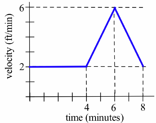
For Problems 19–20, the figure shows your velocity (in feet per minute) along a straight path.

1. Sketch a graph of your location.
2. How many feet did you walk in 8 minutes?
3. Where, relative to your starting location, are you after 8 minutes?

19. See figure below:
    
20. See figure below:
    

Problems 21–27 give the units for \(x\) and \(f(x)\). Specify the units of the definite integral \(\displaystyle \int_a^b f(x)\, dx\).

21. \(x\) is time in “seconds”; \(f(x)\) is velocity in “meters per second”
22. \(x\) is time in “hours”; \(f(x)\) is a flow rate in “gallons per hour”
23. \(x\) a position in “feet”; \(f(x)\) area in “square feet”
24. \(x\) is a time in “days”; \(f(x)\) is a temperature in “degrees Celsius”
25. \(x\) a height in “meters”; \(f(x)\) force in “grams”
26. \(x\) is a position in “inches”; \(f(x)\) is a density in “pounds per inch”
27. \(x\) is a time in “seconds”; \(f(x)\) is an acceleration in “feet per second per second” \(\left(\frac{\mbox{ft}}{\mbox{sec}^2}\right)\)

The remaining problems use the summation formulas given at the end of Section 4.1, as demonstrated in the following Example.

Example \(\PageIndex{8}\)

For \(f(x) = x^2\), divide the interval \([0,2]\) into \(n\) equally wide subintervals, evaluate the lower sum, and compute the limit of that lower sum as \(n \rightarrow\infty\).

Solution

The width of the interval is \(b-a = 2-0 = 2\) so each of the \(n\) subintervals should have width \(\displaystyle \Delta x = \frac{b-a}{n} = \frac{2}{n}\). The endpoints of the \(k\)-th interval in the partition are therefore \((k-1)\cdot \frac{2}{n}\) and \(k\cdot \frac{2}{n}\) for \(k = 1, 2, \ldots, n\).

Because \(f(x) = x^2\) is increasing on \([0,2]\) the minimum value of the function on each subinterval occurs at the left endpoint of the subinterval, hence we need to choose \(c_k = (k-1)\cdot \frac{2}{n}\). So:
\begin{align*}
\mbox{LS} &= \sum_{k=1}^{n}\, f(c_k) \cdot \Delta x_k = \sum_{k=1}^{n}\, \left((k-1)\cdot \frac{2}{n}\right)^2 \cdot \frac{2}{n} = \frac{8}{n^3} \cdot \sum_{k=1}^{n}\, \left(k-1\right)^2\\
&= \frac{8}{n^3} \cdot \sum_{k=1}^{n}\, \left(k^2-2k+1\right) = \frac{8}{n^3}\left[\sum_{k=1}^{n}\, k^2 \ - \ 2 \sum_{k=1}^{n}\, k \ + \ \sum_{k=1}^{n}\, 1\right]\\
&= \frac{8}{n^3}\left[\frac{n(n+1)(2n+1)}{6}-2\cdot\frac{n(n+1)}{2}+n\right] = \frac{8}{n^3}\left[\frac{2n^3-3n^2+n}{6}\right]\\
&= \frac86\left[2 -\frac{3}{n}+\frac{1}{n^2}\right] \end{align*}
As \(n\rightarrow \infty\), LS \(\displaystyle \rightarrow \frac86 (2) = \frac83\) so we can be certain that \(\displaystyle \int_0^2 x^2\, dx \geq \frac83\).

Practice \(\PageIndex{6}\)

Redo Example 8 but find the upper Riemann sum for \(n\) equally wide partition intervals and show that the limit of these upper sums, as \(n\rightarrow\infty\), is \(\displaystyle \frac83\).

Answer

\(\displaystyle \Delta x = \frac{2-0}{n} = \frac{2}{n}\), \(M_k = \frac{2}{n}\cdot k\) so \(f\left(M_k\right) = \left(\frac{2}{n}\cdot k\right)^2 = \frac{4}{n^2}\cdot k^2\). Then:
\begin{align*}\mbox{US} &= \sum_{k=1}^{n}\, f\left(M_k\right)\cdot\Delta x = \sum_{k=1}^{n}\, \frac{4}{n^2}\cdot k^2 \cdot \frac{2}{n}\\
&= \frac{8}{n^3}\sum_{k=1}^{n}\, k^2 = \frac{8}{n^3} \left[\frac13 n^3 + \frac12 n^2 + \frac16 n\right] = \frac83 +\frac{4}{n} + \frac{4}{3n^2}\end{align*}
so the limit of these upper sums as \(n\rightarrow\infty\) is \(\displaystyle \frac83\).

From the previous Example and Practice problem, we know that\[\frac83 \leq \int_0^2 x^2\, dx \leq \frac83\nonumber\]so we can conclude that \(\displaystyle \int_0^2 x^2\, = \frac83\). We will discover a much easier method for evaluating this integral in Section 4.4.

28. For \(f(x) = 3 + x\), partition the interval \([0, 2]\) into \(n\) equally wide subintervals of length \(\Delta x = \frac{2}{n}\).
    1. Compute the lower sum for this function and partition, and calculate the limit of that lower sum as \(n \rightarrow\infty\).
    2. Compute the upper sum for this function and partition and find the limit of the upper sum as \(n \rightarrow\infty\).
29. For \(f(x) = x^3\), partition the interval \([0, 2]\) into \(n\) equally wide subintervals of length \(\Delta x = \frac{2}{n}\).
    1. Compute the lower sum for this function and partition, and calculate the limit of that lower sum as \(n \rightarrow\infty\).
    2. Compute the upper sum for this function and partition and find the limit of the upper sum as \(n \rightarrow\infty\).
30. For \(f(x) = \sqrt{x}\), partition the interval \([0, 9]\) into \(n\) subintervals by taking \(\displaystyle x_k = \frac{9}{n^2}\cdot k^2\) for \(k = 1, 2, \ldots, n\).
    1. Choose \(c_k = x_k\) for each subinterval and compute the upper sum for this function and partition, then calculate the limit of that upper sum as \(n \rightarrow\infty\).
    2. Compute the lower sum for this function and partition and find the limit of the lower sum as \(n \rightarrow\infty\).