4.4: Areas, Integrals and Antiderivatives

This section explores properties of functions defined as areas and examines some connections among areas, integrals and antiderivatives. In order to focus on these connections and their geometric meaning, all of the functions in this section are nonnegative, but in the next section we will generalize (and prove) the results for all continuous functions. This section also introduces examples showing how you can use the relationships between areas, integrals and antiderivatives in various applications.

When \(f\) is a continuous, nonnegative function, the “area function” \(\displaystyle A(x) = \int_{a}^{x} f(t)\, dt\) represents the area of the region bounded by the graph of \(f\), the \(t\)-axis, and vertical lines at \(t=a\) and \(t=x\):

and the derivative of \(A(x)\) represents the rate of change (growth) of \(A(x)\) as the vertical line \(t=x\) moves rightward. Examples 2 and 3 of Section 4.3 showed that for certain functions \(f\), \(A'(x) = f(x)\) so that \(A(x)\) was an antiderivative of \(f(x)\). The next theorem says the result is true for every continuous, nonnegative function \(f\).

Theorem: The Area Function Is an Antiderivative

If: \(f\) is a continuous, nonnegative function and \(\displaystyle A(x) = \int_{a}^{x} f(t)\, dt\) for \(x \geq a\)

then: \(\displaystyle \frac{d}{dx}\left( \int_{a}^{x} f(t)\, dt\right) = A'(x) = f(x)\)

so : \(A(x)\) is an antiderivative of \(f(x)\).

This result relating integrals and antiderivatives is a special case (for nonnegative functions \(f\)) of the first part of the Fundamental Theorem of Calculus (FTC¹), which we will prove in Section 4.5. This result is important for two reasons:

• It says that a large collection of functions have antiderivatives.
• It leads to an easy way to exactly evaluate definite integrals.

Example \(\PageIndex{1}\)

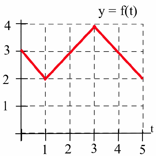
Define \(\displaystyle A(x) = \int_{1}^{x} f(t)\, dt\) for the function \(f(t)\) shown below:

Estimate the values of \(A(x)\) and \(A'(x)\) for \(x = 2\), \(3\), \(4\) and \(5\) and use these values to sketch a graph of \(y = A(x)\).

Solution

Dividing the region into squares and triangles, it is easy to see that \(A(2) = 2\), \(A(3) = 4.5\), \(A(4) = 7\) and \(A(5) = 8.5\). Because \(A'(x) = f(x)\), we know that \(A'(2) = f(2) = 2\), \(A'(3) = f(3) = 3\), \(A'(4) = f(4) = 2\) and \(A'(5) = f(5) = 1\). A graph of \(y = A(x)\) appears below:

It is important to recognize that \(f\) is not differentiable at \(x = 2\) or \(x = 3\) but that the values of \(A\) change smoothly near \(x=2\) and \(x=3\), and the function \(A\) is differentiable at those points and at every other point between \(x=1\) and \(x=5\). Also note that \(f'(4) = -1\) (\(f\) is clearly decreasing near \(x = 4\)) but that \(A'(4) = f(4) = 2\) is positive (the area \(A\) is growing even though \(f\) is getting smaller).

Practice \(\PageIndex{1}\)

Let \(B(x)\) be the area bounded by the horizontal axis, vertical lines at \(t = 0\) and \(t = x\), and the graph of \(f(t)\), shown below:

Estimate the values of \(B(x)\) and \(B'(x)\) for \(x = 1\), \(2\), \(3\), \(4\) and \(5\).

Answer

\(B(1) = 2.5\), \(B(2) = 5\), \(B(3) = 8.5\), \(B(4) = 12\), \(B(5) = 14.5\)

\(\displaystyle B(x) = \int_0^{x} f(t)\, dt \ \Rightarrow \ B'(x) = \frac{d}{dx}\left( \int_0^{x} f(t)\, dt \right) = f(x)\) (by the Area Function Is an Antiderivative Theorem), hence: \(B'(1) = f(1) = 2\), \(B'(2) = f(2) = 3\), \(B'(3) = 4\), \(B'(4) = 3\) and \(B'(5) = 2\).

Example \(\PageIndex{2}\)

Let \(\displaystyle G(x) = \frac{d}{dx}\left(\int_{0}^{x} \sin(t)\, dt\right)\). Evaluate \(G(x)\) for \(\displaystyle x = \frac{\pi}{4}\), \(\displaystyle \frac{\pi}{2}\) and \(\displaystyle \frac{3\pi}{4}\).

Solution

The figure below shows \(\displaystyle A(x) = \int_{0}^{x} \sin(t)\, dt\) graphically:

By the theorem, \(A'(x) = \sin(x)\), so:
\begin{align*}
G\left(\frac{\pi}{4}\right) = A'\left(\frac{\pi}{4}\right) &= \sin\left(\frac{\pi}{4}\right) = \frac{1}{\sqrt{2}} \approx 0.707\\
G\left(\frac{\pi}{2}\right) = A'\left(\frac{\pi}{2}\right) &= \sin\left(\frac{\pi}{2}\right) = 1\\ 
G\left(\frac{3\pi}{4}\right) = A'\left(\frac{3\pi}{4}\right) &= \sin\left(\frac{3\pi}{4}\right) = \frac{1}{\sqrt{2}} \approx 0.707\end{align*}
The next figure shows a graph of \(y = A(x)\):

and this figure shows the graph of \(y = A'(x) = G(x)\):

 

Using Antiderivatives to Evaluate \(\displaystyle\int_{a}^{b} f(x)\, dx\)

Now we combine the ideas of areas and antiderivatives to devise a technique for evaluating definite integrals that is exact — and often easy.

If \(\displaystyle A(x) = \int_{a}^{x} f(t)\, dt\), then we know that \(\displaystyle A(a) = \int_{a}^{a} f(t)\, dt = 0\), \(\displaystyle A(b) = \int_{a}^{b} f(t)\, dt\) and that \(A(x)\) is an antiderivative of \(f\), so \(A'(x) = f(x)\). We also know that if \(F(x)\) is any antiderivative of \(f\), then \(F(x)\) and \(A(x)\) have the same derivative so \(F(x)\) and \(A(x)\) are “parallel” functions and differ by a constant: \(F(x) = A(x) + C\) for all \(x\) and some constant \(C\). As a consequence:
\begin{align*}F(b) - F(a) &= \left[ A(b) + C \right] - \left[A(a) + C \right] = A(b) - A(a)\\
                          &= \int_{a}^{b} f(t)\, dt -  \int_{a}^{a} f(t)\, dt = \int_{a}^{b} f(t)\, dt \end{align*}
This result says that, to evaluate a definite integral \(\displaystyle A(b) = \int_{a}^{b} f(t)\, dt\), we can find any antiderivative \(F\) of \(f\) and simply evaluate \(F(b) - F(a)\). 

This result is a special case of the second part of the Fundamental Theorem of Calculus (FTC²), stated and proved in Section 4.5), which you will use hundreds of times over the next several chapters.  

Theorem: Antiderivatives and Definite Integrals

If: \(f\) is a continuous, nonnegative function and \(F\) is any antiderivative of \(f\) (so that \(F'(x) = f(x)\)) on \([a,b]\)

then: \(\displaystyle \int_{a}^{b} f(t)\, dt = F(b) - F(a)\)

The problem of finding the exact value of a definite integral has been reduced to finding some (any) antiderivative \(F\) of the integrand and then evaluating \(F(b) - F(a)\). Even finding one antiderivative can be difficult, so for now we will restrict our attention to functions that have “easy” antiderivatives. Later we will explore some methods for finding antiderivatives of more “difficult” functions.

Because an evaluation of the form \(F(b) - F(a)\) will occur quite often, we represent it symbolically as \(\displaystyle F(x) \Big|_a^b\) or \(\displaystyle {\Big[}F(x){\Big]}_a^b\).

Example \(\PageIndex{3}\)

Evaluate \(\displaystyle \int_1^3 x\ dx\) in two ways:

1. by sketching a graph of \(y = x\) and finding the area represented by the definite integral.
2. by finding an antiderivative \(F(x)\) of \(f(x)=x\) and evaluating \(F(3)-F(1)\).

Solution

1. A graph of \(y = x\) appears below:
   
   the area of the trapezoidal region in question has area \(4\).
2. One antiderivative of \(x\) is \(\displaystyle F(x) = \frac12 x^2\) (you should check for yourself that \(\displaystyle \mbox{D}\left(\frac{x^2}{2}\right) = x\)), so:\[F(x) \Bigg|_1^3 = F(3)-F(1) = \frac12 (3)^2 - \frac12 (1)^2 = \frac92 - \frac12 = 4\nonumber\]which agrees with the area from part (a).

If someone chose another antiderivative of \(x\), say \(F(x) = \frac12 x^2 + 7\) (you should check for yourself that \(\displaystyle \mbox{D}\left(\frac{x^2}{2} + 7\right) = x\)), then:\[F(x) \Bigg|_1^3 = F(3)-F(1) = \left[\frac12 (3)^2 + 7\right] - \left[\frac12 (1)^2 +7\right] = \frac{23}{2} - \frac{15}{2} = 4\nonumber\]No matter which antiderivative \(F\) we choose, \(F(3) - F(1) = 4\).

Practice \(\PageIndex{2}\)

Evaluate \(\displaystyle \int_1^3 (x-1)\, dx\) in the two ways specified in the previous Example.

Answer

1. \(\displaystyle \int_1^3 \left(x - 1\right)\, dx\) gives the area of the triangular region between the graph of \(y = x - 1\) and the \(x\)-axis for \(1 \leq x \leq 3\):\[\mbox{area} = \frac12 \left(\mbox{base}\right)\left(\mbox{height}\right) = \frac12 (2)(2) = 2\nonumber\]
2. \(F(x) = \frac12 x^2 - x\) is an antiderivative of \(f(x) = x - 1\) so:\[\int_1^3 \left(x - 1\right)\, dx  = F(3) - F(1) = \left[\frac12 \cdot 3^3 - 3\right] - \left[\frac12 \cdot 1^3 - 1\right] = 2\nonumber\]

This antiderivative method provides an extremely powerful way to evaluate some definite integrals, and we will use it often.

Example \(\PageIndex{4}\)

Find the area of the region in the first quadrant bounded by the graph of \(y = \cos(x)\), the horizontal axis, and the vertical line \(x=0\).

Solution

The area we want:

is \(\displaystyle \int_0^{\frac{\pi}{2}} \cos(x)\, dx\) so we need an antiderivative of \(f(x) = \cos(x)\). \(F(x) = \sin(x)\) is one such antiderivative (you should check that \(\mbox{D}\left(\sin(x)\right) = \cos(x)\)), so\[\int_0^{\frac{\pi}{2}} \cos(x)\, dx = \sin(x)\bigg|_0^{\frac{\pi}{2}} = \sin\left(\frac{\pi}{2}\right) - \sin(0) = 1- 0 = 1\nonumber\]is the area of the region in question.

Practice \(\PageIndex{3}\)

Find the area of the region bounded by the graph of \(y = 3x^2\), the horizontal axis and the vertical lines \(x =1\) and \(x=2\).

Answer

Area \(\displaystyle = \int_1^2 3x^2\, dx = x^3 \bigg|_1^2 = 2^3-1^3 = 8 - 1 = 7\)

Integrals, Antiderivatives and Applications

The antiderivative method for evaluating definite integrals can also be used when we need to find a more general “area,” so it is often useful for solving applied problems.

Example \(\PageIndex{5}\)

A robot has been programmed so that when it starts to move, its velocity after \(t\) seconds will be \(3t^2\) feet per second.

1. How far will the robot travel during its first four seconds of movement? 
2. How far will the robot travel during its next four seconds of movement? 
3. How long will it take for the robot to move 729 feet from its starting place? 

Solution

1. The distance during the first four seconds will be the area under the graph of the velocity function:
   
   from \(t = 0\) to \(t = 4\), an area we can compute with the definite integral \(\displaystyle \int_0^4 3t^2 \, dt\). One antiderivative of \(3t^2\) is \(t^3\) so:\[\int_0^4 3t^2 \, dt = \left[t^3\right]_0^4 = 4^3-0^3 = 64\nonumber\]and we can conclude that the robot will be 64 feet away from its starting position after four seconds.
2. Proceeding similarly:\[\int_4^8 3t^2 \, dt = \left[t^3\right]_4^8 = 8^3-4^3 = 512-64 = 448\,\mbox{feet}\nonumber\]
3. This question is different from the first two. Here we know the lower integration endpoint, \(t = 0\), and the total distance, 729 feet, and need to find the upper integration endpoint (the time when the robot is 729 feet away from its starting position). Calling this upper endpoint \(T\), we know that:\[729 = \int_0^T 3t^2 \, dt = \left[t^3\right]_0^T = T^3-0^3 = T^3\nonumber\]so \(T = \sqrt[3]{729} = 9\). The robot is 729 feet away after 9 seconds. 

Practice \(\PageIndex{4}\)

Refer to the robot from Example \(\PageIndex{5}\).

1. How far will the robot travel between \(t = 1\) and \(t = 5\) seconds? 
2. How long will it take for the robot to move 343 feet from its starting place? 

Answer

1. distance \(\displaystyle = \int_1^5 3t^2\, dt = t^3\Big|_1^5 = 125- 1 = 124\) feet. 
2. We know the starting point is \(x = 0\) and the total distance (“area” under the velocity curve) is 343 feet. We need to find the time \(T\):
   
   so that 343 feet \(\displaystyle = \int_0^T 3t^2\, dt\):\[343 = \int_0^T 3t^2\, dt = t^3\bigg|_0^T = T^3 - 0 = T^3\nonumber\]hence \(T = \sqrt[3]{343} = 7\) seconds.

Example \(\PageIndex{6}\)

Suppose that \(t\) minutes after placing 1,000 bacteria on a Petri plate the rate of growth of the bacteria population is \(6t\) bacteria per minute.

1. How many new bacteria are added to the population during the first seven minutes?
2. What is the total population after seven minutes?
3. When will the total population reach 2,200 bacteria? 

Solution

1. The number of new bacteria is represented by the area under the rate-of-growth graph:
   
   and one antiderivative of \(6t\) is \(3t^2\) (check that \(\mbox{D}\left(3t^2\right) = 6t\)) so:\[\mbox{new bacteria} = \int_0^7 6t\, dt = \left[3t^2\right]_0^7 = 3(7)^2-3(0)^2 = 147\nonumber\]
2. \(\left[\mbox{old population}\right] + \left[\mbox{new bacteria}\right] = 1000 + 147 = 1147\,\mbox{bacteria}\).
3. When the total population reaches 2,200 bacteria, then there are \(2200 - 1000 = 1200\) new bacteria, hence we need to find the time \(T\) required for that many new bacteria to grow:\[1200 = \int_0^T 6t\, dt = \left[3t^2\right]_0^T = 3(T)^2 - 3(0)^2 = 3T^2\nonumber\]so \(T^2 = 400 \Rightarrow T = 20\). After 20 minutes, the total bacteria population will be \(1000 + 1200 = 2200\).

Practice \(\PageIndex{5}\)

Refer to the bacteria population from the previous Example.

1. How many new bacteria will be added to the population between \(t = 4\) and \(t = 8\) minutes?  
2. When will the total population reach 2,875 bacteria? 

Answer

1. new bacteria \(\displaystyle = \int_4^8 6t\, dt = 3t^2\bigg|_4^8 = 3\cdot 64 - 3\cdot 16 = 144\) bacteria. 
2. We know the total new population (“area” under the rate-of-change graph):
   
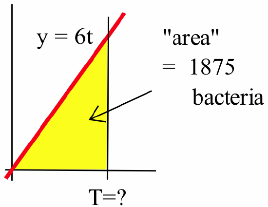
   is \(2875 - 1000 = 1875\) so:\[1875 = \int_0^T 6t\, dt = 3t^2\bigg|_0^T = 3T^2 - 0 = 3T^2 \ \Rightarrow \ T^2 = 625\nonumber\]hence \(T = \sqrt{625} = 25\) minutes.

Problems

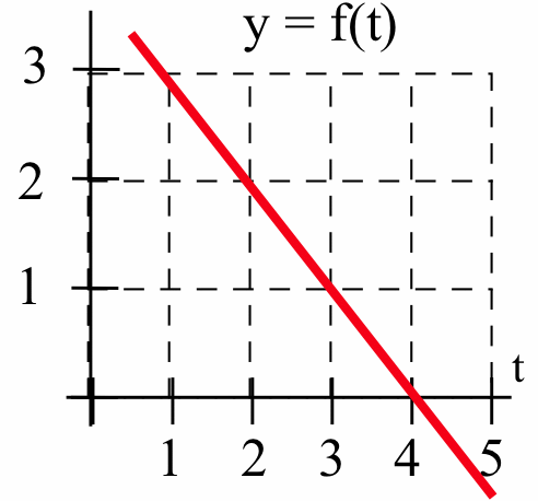
In Problems 1–8, \(\displaystyle A(x) = \int_{1}^{x} f(t)\, dt\) with \(f(t)\) given.

1. Graph \(y = A(x)\) for \(1 \leq x \leq 5\).
2. Estimate the values of \(A(1)\), \(A(2)\), \(A(3)\) and \(A(4)\).
3. Estimate \(A'(1)\), \(A'(2)\), \(A'(3)\) and \(A'(4)\).

1. 
2. 
3. 
4. 
5. \(f(t) = 2\)
6. \(f(t) = 1 + t\)
7. \(f(t) = 6 - t\)
8. \(f(t) = 1 + 2t\)

In Problems 9–18, use the Antiderivatives and Definite Integrals Theorem to evaluate each integral.

9. 1. \(\displaystyle \int_0^3 2x\, dx\)
   2. \(\displaystyle \int_1^3 2x\, dx\)
   3. \(\displaystyle \int_0^1 2x\, dx\)
10. 1. \(\displaystyle \int_0^2 4x^3\, dx\)
    2. \(\displaystyle \int_0^1 4x^3\, dx\)
    3. \(\displaystyle \int_1^2 4x^3\, dx\)
11. 1. \(\displaystyle \int_1^3 6x^2\, dx\)
    2. \(\displaystyle \int_1^2 6x^2\, dx\)
    3. \(\displaystyle \int_0^3 6x^2\, dx\)
12. 1. \(\displaystyle \int_{-2}^2 2x\, dx\)
    2. \(\displaystyle \int_{-2}^{-1} 2x\, dx\)
    3. \(\displaystyle \int_{-2}^0 2x\, dx\)
13. 1. \(\displaystyle \int_0^3 4x^3\, dx\)
    2. \(\displaystyle \int_1^3 4x^3\, dx\)
    3. \(\displaystyle \int_0^1 4x^3\, dx\)
14. 1. \(\displaystyle \int_0^5 4x^3\, dx\)
    2. \(\displaystyle \int_0^2 4x^3\, dx\)
    3. \(\displaystyle \int_2^5 4x^3\, dx\)
15. 1. \(\displaystyle \int_{-3}^3 3x^2\, dx\)
    2. \(\displaystyle \int_{-3}^0 3x^2\, dx\)
    3. \(\displaystyle \int_0^3 3x^2\, dx\)
16. 1. \(\displaystyle \int_0^3 5\, dx\)
    2. \(\displaystyle \int_0^2 5\, dx\)
    3. \(\displaystyle \int_2^3 5\, dx\)
17. 1. \(\displaystyle \int_0^2 3x^2\, dx\)
    2. \(\displaystyle \int_1^3 3x^2\, dx\)
    3. \(\displaystyle \int_3^1 3x^2\, dx\)
18. 1. \(\displaystyle \int_{-2}^2 \left[12-3x^2\right]\, dx\)
    2. \(\displaystyle \int_0^2 \left[12-3x^2\right]\, dx\)
    3. \(\displaystyle \int_1^2 \left[12-3x^2\right]\, dx\)

In 19–21, use the given velocity of a car (in feet per second) after \(t\) seconds to find:

1. how far the car travels during the first 10 seconds.
2. how many seconds it takes the car to travel half the distance in part (a).

19. \(v(t) = 2t\) 
20. \(v(t) = 3t^2\) 
21. \(v(t) = 4t^3\) 

Problems 22–23 give the velocity of a car (in feet per second) after \(t\) seconds.

1. How many seconds does it take for the car to come to a stop (velocity \(= 0\))?
2. How far does the car travel before coming to a stop? 
3. How many seconds does it take the car to travel half the distance in part (b)?

22. \(v(t) = 20-2t\)
23. \(v(t) = 75-3t^2\)
24. Find the exact area under half of one arch of the sine curve: \(\displaystyle \int_0^{\frac{\pi}{2}} \sin(x)\, dx\).
25. An artist you know wants to make a figure consisting of the region between the curve \(y = x^2\) and the \(x\)-axis for \(0\leq x \leq 3\).
    1. Where should the artist divide the region with a vertical line:
       
       so that each piece has the same area?
    2. Where should she divide the region with vertical lines to get three pieces with equal areas?