4.7: First Applications of Definite Integrals

The development of calculus by Newton and Leibniz was a vital step in the advancement of pure mathematics, but Newton also advanced the sciences and applied mathematics. Not only did he discover theoretical results, he immediately used those results to answer important questions about gravity and motion. The success of these applications of mathematics to the physical sciences helped establish what we now take for granted: mathematics can and should be used to answer questions about the world.

Newton applied mathematics to the outstanding problems of his day, problems primarily in the field of physics. During the intervening 300-plus years, thousands upon thousands of people have continued these theoretical and applied traditions, using mathematics to help develop our understanding of the physical and biological sciences, as well as the behavioral sciences and economics. Mathematics is still used to answer new questions in physics and engineering, but it is also important for modeling ecological processes, for understanding the behavior of DNA, for determining how the brain works, and even for devising financial strategies. The mathematics you are learning now can help you become part of this tradition, and you might even use it to add to our understanding of the world.

It is important to understand the special applications of integration we will study in case you need to use those particular applications. But it is also important that you understand the process of building models with integrals so you can apply that process to other situations in a variety of fields of study. Conceptually, converting an applied problem to a Riemann sum is the most valuable step. (Typically, it is also the most challenging.)

Area between Two Curves

We have already used integrals to find the area between the graph of a function and the horizontal axis. We can also use integrals to find the area between the graphs of two functions.

If \(f(x) \geq g(x)\) for all \(x\) in \([a,b]\), then we can approximate the area between the graphs of \(f\) and \(g\) by partitioning the interval \([a,b]\) and forming a Riemann sum:

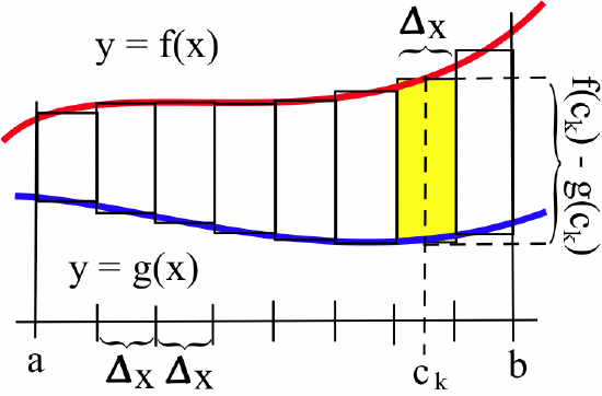
The height of each rectangle is \(f(c_k) - g(c_k)\) so the area of the \(k\)-th rectangle is:\[(\mbox{height})\cdot(\mbox{base}) = \left[f(c_k) - g(c_k)\right]\cdot \Delta x_k\nonumber\]and an approximation of the total area is given by\[\sum_{k=1}^{n} \left[f(c_k) - g(c_k)\right]\cdot\Delta x_k\nonumber\]which is a Riemann sum.

The limit of this Riemann sum, as the mesh of the partitions approaches \(0\), is a definite integral:\[\int_a^b \left[f(x)-g(x)\right]\, dx\nonumber\]We will sometimes use an arrow to indicate “the limit of the Riemann sum as the mesh of the partitions approaches \(0\),” writing:\[\sum_{k=1}^{n} \left[f(c_k) - g(c_k)\right]\cdot\Delta x_k \ \longrightarrow \ \int_a^b \left[f(x)-g(x)\right]\, dx\nonumber\]

If: \(T(x) \geq B(x)\) for \(a \leq x \leq b\)

then: the area of the region bounded by the graphs of the “top” function \(T(x)\), the “bottom” function \(B(x)\), and the lines \(x=a\) and \(x=b\) is given by:\[\int_a^b \left[T(x)-B(x)\right] \, dx\nonumber\]

Example \(\PageIndex{1}\)

Find the area bounded between the graphs of \(f(x) = x\) and \(g(x) = 3\) for \(1 \leq x \leq 4\).

Solution

It is clear from the figure below:

that the area between \(f\) and \(g\) is \(2.5\) square units. Using the integration procedure above, we need to identify a “top” function and a “bottom” function. For \(1\leq x \leq 3\), \(g(x) = 3 \geq x = f(x)\) so the area of the left-hand triangle is given by the integral:\[\int_1^3 \left[3-x\right]\, dx = \left[3x-\frac12 x^2\right]_1^3 = \left[9-\frac92\right]-\left[3-\frac12\right] = 2\nonumber\]For the interval \(3\leq x \leq 4\), \(g(x) = 3 \leq x = f(x)\) so the area of the right-hand triangle is given by the integral:\[\int_3^4 \left[x-3\right]\, dx = \left[\frac12 x^2-3x\right]_3^4 = \left[8-12\right]-\left[\frac92-9\right] = \frac12\nonumber\]Adding these two areas, we get \(2 + 0.5 = 2.5\).

If we had mindlessly integrated in the previous Example without consulting a graph:\[\int_1^4 \left[3-x\right]\, dx = \left[3x-\frac12 x^2\right]_1^4 = \left[12-8\right]-\left[3-\frac12\right] = \frac32\nonumber\]we would have arrived at an incorrect answer.

Graphing the region in question to determine which function is on “top” and which is on “bottom” is often crucial to getting the right answer to a problem involving the area between two curves.

Practice \(\PageIndex{1}\)

Use integrals and the graphs of \(f(x) = 1 + x\) and \(g(x) = 3 - x\) to determine the area between the graphs of \(f\) and \(g\) for \(0 \leq x \leq 3\).

Answer

Referring to a graph:

and using geometry: \)\displaystyle A = \frac12(2)(1) = 1\) and \(\displaystyle B = \frac12(4)(2) = 4\) so the total area is \(1+4=5\). 

Referring to a graph of the functions and using integrals:
\begin{align*}A &= \int_0^1 \left[(3-x) - (1+x)\right]\, dx = \int_0^1 \left[2-2x\right]\, dx\\
&= \left[2x - x^2\right]_0^1 = \left[2-1\right] - \left[0-0\right] = 1\\
B &= \int_1^3 \left[(1+x) - (3-x)\right]\, dx = \int_1^3 \left[2x - 2\right]\, dx\\
&= \left[x^2 - 2x\right]_1^3 = \left[9 - 6\right] - \left[1 - 2)\right] = 4\end{align*}
which also results in a total area of \(1+4=5\).

Example \(\PageIndex{2}\)

Objects \(A\) and \(B\) start from the same location at the same time and travel along the same path with respective velocities \(v_A(t) = t + 3\) and \(v_B(t) = t^2 - 4t + 3\) meters per second:

How far ahead is \(A\) after 3 seconds? After 5 seconds?

Solution

From the graph, it appears that \(v_A(t) \geq v_B(t)\), at least for \(0\leq t \leq 3\), but for the second question we need to know whether this holds for \(3\leq t \leq 5\) as well. Setting \(v_A(t) = v_B(t)\) to see where the graphs intersect:\[t+3 = t^2-4t+3 \quad \Rightarrow \quad t^2-5t = 0 \quad \Rightarrow \quad t=0 \ \mbox{ or } \ t = 5\nonumber\]Checking that \(v_A(1) = 4 > 0 = v_B(1)\) (or referring to the graph), we can conclude that \(v_A(t) \geq v_B(t)\) on the interval \([0,5]\).

Because \(v_A(t) \geq v_B(t)\), the “area” between the graphs of \(v_A\) and \(v_B\) over an interval \([0,x]\) represents the distance between the objects after \(x\) seconds. After three seconds, the distance apart is:
\begin{align*}\int_0^3 \left[v_A(t)-v_B(t)\right]\, dt &= \int_0^3 \left[(t+3)-(t^2-4t+3)\right]\, dt = \int_0^3\left[5t-t^2\right]\, dt\\
&= \left[\frac52 t^2 - \frac13 t^3 \right]_0^3 = \left[\frac{45}{2}-9\right]-\left[0-0\right] = \frac{27}{2}\end{align*}
or 13.5 meters. After five seconds, the distance apart is\[\int_0^5 \left[v_A(t)-v_B(t)\right]\, dt = \left[\frac52 t^2 - \frac13 t^3 \right]_0^5 = \frac{125}{6}\nonumber\]or approximately 20.83 meters.

If \(f(x) \geq g(x) \geq 0\) on an interval \([a,b]\), as illustrated in the figure below:

we could have used a simpler geometric argument that the area between the graphs of \(f\) and \(g\) is just the area below the graph of \(f\) minus the area below the graph of \(g\):\[\int_a^b f(x) \, dx - \int_a^b g(x) \, dx = \int_a^b\left[f(x)-g(x)\right]\, dx\nonumber\]which agrees with our previous result. We took a different approach at the beginning of this section, however, because it provides a nice (yet simple) example of translating a geometric or physical problem into a Riemann sum and then into a definite integral.

Example \(\PageIndex{3}\)

Find the area of the shaded region in the figure below:

Solution

These are the same two functions from our previous Example; in our previous solution we observed that \(t+3 \geq t^2-4t+3\) for \(0 \leq t \leq 5\), and it is straightforward to check that \(t+3 \leq t^2-4t+3\) for \(t \geq 5\) (and, in particular, for \(5 \leq t \leq 7\)).

We therefore need to split our problem into two pieces and subtract the “bottom” function from the “top” function on each interval. The area of the left region is:\[\int_0^5 \left[(t+3)-(t^2-4t+3)\right]\, dt = \left[\frac52 t^2 - \frac13 t^3 \right]_0^5 = \frac{125}{6}\nonumber\](as worked out in the previous example), while the area of the region on the right is:\[\int_5^7 \left[(t^2-4t+3)-(t+3)\right]\, dt = \left[\frac13 t^3 - \frac52 t^2\right]_5^7 = \frac{38}{3}\nonumber\]so the total area is \(\displaystyle \frac{125}{6}+\frac{38}{3} = \frac{67}{2} = 33.5\).

Average Value of a Function

We compute the average (or mean value) of \(n\) numbers, \(a_1, a_2,\ldots , a_n\) by adding them up and dividing by \(n\):\[\mbox{average} = \overline{a} = \frac{1}{n}\sum_{k=1}^{n} \, a_k\nonumber\]but computing the average value of a function requires an integral. (A “bar” above a quantity typically indicates the mean of that quantity.)

To estimate the average value of \(f\) on the interval \([a,b]\), we can partition \([a,b]\) into \(n\) equally long subintervals of length \(\displaystyle \Delta x =\frac{b-a}{n}\), then choose a value \(c_k\) in each subinterval, and find the average of the function values \(f(c_k)\) at those \(n\) points:\[\overline{f} = \mbox{average of } f \ \approx  \ \frac{f(c_1)+f(c_2)+\cdots +f(c_n)}{n} \ = \ \sum_{k=1}^{n} \, f(c_k)\cdot \frac{1}{n}\nonumber\]While this last term resembles a Riemann sum, it does not have the form \(\displaystyle \sum f(c_k)\cdot \Delta x_k\), because \(\displaystyle \frac{1}{n} \neq \Delta x = \frac{b-a}{n}\). But multiplying and dividing by \(b-a\) yields:\[\sum_{k=1}^{n} \, f(c_k)\cdot \frac{1}{n} = \sum_{k=1}^{n} \, f(c_k)\cdot \frac{b-a}{n}\cdot\frac{1}{b-a} = \frac{1}{b-a} \sum_{k=1}^{n} \, f(c_k)\cdot \frac{b-a}{n}\nonumber\]This last (Riemann) sum converges to a definite integral:\[\frac{1}{b-a} \sum_{k=1}^{n} \, f(c_k)\cdot \frac{b-a}{n} = \frac{1}{b-a} \sum_{k=1}^{n} \, f(c_k)\cdot \Delta x \longrightarrow \frac{1}{b-a} \int_a^b f(x) \, dx\nonumber\]as the number of subintervals \(n\) gets larger and the mesh, \(\displaystyle \Delta x = \frac{b-a}{n}\), approaches \(0\).

Definition: Average (Mean) Value of a Function

The average value of an integrable function \(f\) on \([a,b]\) is \[\frac{1}{b-a} \int_a^b f(x) \, dx\]

The average value of a positive function has a nice geometric interpretation. Imagine that the area under \(f\) represents a liquid trapped above by the graph of \(f\) and on the other sides by the \(x\)-axis and the lines \(x=a\) and \(x=b\):

If we remove the “lid” (the graph of \(f\)), the liquid would settle into the shape of a rectangle with the same area as the region under the graph of \(f\). If the height of this rectangle is \(H\), then the area of the rectangle is \(H\cdot(b-a)\), so:\[H\cdot(b-a) = \int_a^b f(x) \, dx \quad \Rightarrow \quad H = \frac{1}{b-a} \int_a^b f(x) \, dx\nonumber\]The average value of a positive function \(f\) is the height \(H\) of the rectangle whose area is the same as the area under \(f\).

Example \(\PageIndex{4}\)

Find the average value of \(\sin(x)\) on the interval \([0,\pi]\).

Solution

Using our definition, the average value is:\[\frac{1}{\pi-0} \int_0^{\pi} \sin(x) \, dx = \frac{1}{\pi} \Big[-\cos(x)\Big]_0^{\pi} = \frac{1}{\pi} [(1)-(-1)] = \frac{2}{\pi} \approx 0.6366\nonumber\]A rectangle with height \(\displaystyle\frac{2}{\pi} \approx 0.64\) on the interval \([0,\pi]\) encloses the same area as one arch of the sine curve.

If the interval in the previous Example had been \([0, 2\pi]\), the average value would be \(0\). (Why?)

Practice \(\PageIndex{2}\)

During a nine-hour work day, the production rate at time \(t\) hours was \(r(t)= 5 + \sqrt{t}\) cars per hour. Find the average hourly production rate.

Answer

Using the average value formula:
\begin{align*}\frac{1}{9-0} \int_0^9 \left[5 + \sqrt{t}\right]\, dt &= \frac19 \int_0^9 \left[5 + t^{\frac12}\right]\, dt = 
\frac19 \left[5t + \frac23 t^{\frac32}\right]_0^9\\
&= \frac19\left[\left(45 + \frac23\cdot 27\right) - (0+0)\right] = \frac{45 + 18}{9} = 7\end{align*}
so the average hourly production rate is 7 cars per hour.

Function averages, involving means as well as more complicated techniques, are used to “smooth” data so that underlying patterns become more obvious and to remove high frequency “noise” from signals. In these situations, the value of the original function \(f\) at a point is replaced by some “average of \(f\)” over an interval including that point. If \(f\) is the graph of rather jagged data:

then the 10-year average of \(f\) is the integral:\[g(x) = \frac{1}{10}\int_{x-5}^{x+5} f(t)\, dt\nonumber\]an average of \(f\) over a timespan of five years on either side of \(x\).

The figure below shows the graphs of a monthly average (rather “noisy” data) of surface-temperature data, an annual average (still rather “jagged”) and a five-year average (a much smoother function):

Typically this “moving average” function reveals a pattern much more clearly than the original data. (This “moving average” of “noisy” data is frequently used with data such as weather information and stock prices.)

Work

In physics, the amount of work done on an object is defined as the force applied to the object times the displacement of the object (the distance the object is moved while the force is applied). Or, more succinctly:

Definition

\(\mbox{work} = (\mbox{force})\cdot(\mbox{displacement})\)

If you lift a three-pound book two feet, then the force is \(3\) pounds (the weight of the book), and the displacement is \(2\) feet, so you have done \((3\mbox{ pounds})\cdot(2\mbox{ feet}) = 6\) foot-pounds of work. 

When the applied force and the displacement are both constants, calculating work is simply a matter of multiplication. 

Practice \(\PageIndex{3}\)

How much work is done lifting a 10-pound object from the ground to the top of a 30-foot building?

Answer

\((\mbox{force})\cdot(\mbox{displacement}) = (10\mbox{ pounds})\cdot(30\mbox{ feet}) = 300\mbox{ foot-pounds}\)

If either the force or the displacement varies, however, we need to use integration.

Example \(\PageIndex{5}\)

How much work is done lifting a 10-pound object from the ground to the top of a 30-foot building using a cable that weighs \(2\) pounds per foot?

Solution

This is more challenging situation. We know the work needed to move the object is \((10)(30) = 300\) foot-pounds, but once we start pulling the cable onto the roof, we need to do less and less work to pull the remaining part of the cable.

Let’s partition the cable into small increments so the displacement of each small piece of the cable is roughly constant.

If we break the cable into \(n\) small pieces, each piece has length \(\displaystyle \Delta x = \frac{30}{n}\), so its weight (the force required to move it) is:\[\left(\Delta x \mbox{ ft}\right)\cdot \left(2 \ \frac{\mbox{lbs}}{\mbox{ft}} \right) = 2\Delta x \mbox{ lbs}\nonumber\]If this small piece of cable is initially \(c_k\) feet above the ground, then its displacement is \(30-c_k\) feet, so the work done on this small piece is \(2(30-c_k) \Delta x\) ft-lbs and the total work done on the entire cable is (approximately):\[\sum_{k=1}^{n} \, 2(30-c_k)\Delta x \quad \longrightarrow \quad \int_0^{30} 2(30-x)\, dx\nonumber\]Once again we have formed a Riemann sum, which converges to a definite integral as we chop the cable into smaller and smaller pieces. This integral represents the work needed to lift the cable to the roof: \begin{align*}\int_0^{30} 2(30-x)\, dx &= \int_0^{30} (60-2x)\, dx = 60x-x^2\bigg|_0^{30}\\ &= \left[1800-900\right]-\left[0-0\right] = 900 \mbox{ ft-lbs}\end{align*} so the total work required to lift the object and the cable to the roof is \(300+900 =1200\) ft-lbs.

Practice \(\PageIndex{4}\)

Suppose the building in Example 5 is 50 feet tall and the cable weighs 3 pounds per foot.

1. Compute the work done raising the object from the ground to a height of 10 feet.
2. From a height of 10 feet to a height of 20 feet.

Answer

1. The work required to move the object a distance of 10 feet is \((10\mbox{ pounds})\cdot(10\mbox{ feet}) = 100\mbox{ foot-pounds}\). The work required to move the top 10 feet of the cable onto the roof is:\[\int_0^{10} \left(10-x\right)\cdot 3\, dx = \left[30x-\frac32 x^2\right]_0^{10} = \left[300-150\right]-\left[0\right] = 150 \mbox{ ft-lbs}\nonumber\]and the force required to move the remaining 40 feet of cable is:\[(40\mbox{ ft})\cdot\left(3 \ \frac{\mbox{lbs}}{\mbox{ft}}\right)\left(10\mbox{ ft}\right) = 1200\mbox{ ft-lbs}\nonumber\]so the total work required is \(100+150+1200 = 1450\) foot-pounds.
2.  
3. The work required to move the object a distance of 10 feet is again \((10\mbox{ pounds})\cdot(10\mbox{ feet}) = 100\mbox{ foot-pounds}\). The work required to move the top 10 feet of the cable onto the roof is again \(150\) foot-pounds, and the force required to move the remaining 30 feet of cable is:\[(30\mbox{ ft})\cdot\left(3 \ \frac{\mbox{lbs}}{\mbox{ft}}\right)\left(10\mbox{ ft}\right) = 900\mbox{ ft-lbs}\nonumber\]so the total work required is \(100+150+900 = 1150\) foot-pounds.

The situation in the previous Example and Practice problems is but one of many that arise when computing work. We will examine others in Section 5.4.

Summary

The area, average and work applications in this section merely introduce a few of the many applications of definite integrals. They illustrate the pattern of moving from an applied problem to a Riemann sum, to a definite integral and, finally, to a numerical answer. We will explore many more applications in Chapter 5.

Problems

In Problems 1–4, use the values in the table below to estimate the indicated areas.

\(x\)	\(f(x)\)	\(g(x)\)	\(h(x)\)
0	5	2	5
1	6	1	6
2	6	2	8
3	4	2	6
4	3	3	5
5	2	4	4
6	2	5	2

1. Estimate the area between \(f\) and \(g\) for \(1 \leq x \leq 4\).
2. Estimate the area between \(f\) and \(g\) for \(1 \leq x \leq 6\).
3. Estimate the area between \(f\) and \(h\) for \(0 \leq x \leq 4\).
4. Estimate the area between \(g\) and \(h\) for \(0 \leq x \leq 6\).
5. Estimate the area of the island in the figure below:
   
6. Estimate the area of the island in figure above if the distances between the lines is 50 feet instead of 40 feet.

In Problems 7–18, sketch a graph of each function and find the area between the graphs of \(f\) and \(g\) for \(x\) in the given interval.

7. \(f(x) = x^2 + 3\), \(g(x) = 1\), \(-1 \leq x \leq 2\)
8. \(f(x) = x^2 + 3\), \(g(x) = 1+x\), \(0 \leq x \leq 3\)
9. \(f(x) = x^2\), \(g(x) = x\), \(0 \leq x \leq 2\)
10. \(f(x) = 4 - x^2\), \(g(x) = x + 2\), \(0 \leq x \leq 2\)
11. \(\displaystyle f(x) = \frac{1}{x}\), \(g(x) = x\), \(1 \leq x \leq e\)
12. \(f(x) = \sqrt{x}\), \(g(x) = x\), \(0 \leq x \leq 4\)
13. \(f(x) = x+1\), \(g(x) = \cos(x)\), \(\displaystyle 0 \leq x \leq \frac{\pi}{4}\)
14. \(f(x) = (x-1)^2\), \(g(x) = x+1\), \(0 \leq x \leq 3\)
15. \(f(x) = e^x\), \(g(x) = x\), \(0 \leq x \leq 2\)
16. \(f(x) = \cos(x)\), \(g(x) = \sin(x)\), \(\displaystyle 0 \leq x \leq \frac{\pi}{4}\)
17. \(f(x) = 3\), \(g(x) = \sqrt{1-x^2}\), \(0 \leq x \leq 1\)
18. \(f(x) = 2\), \(g(x) = \sqrt{4-x^2}\), \(-2 \leq x \leq 2\)

In Problems 19–22, use the values of \(f\) in the table at the beginning of the page to estimate the average value of \(f\) on the indicated interval.

19. \([0.5, 4.5]\)
20. \([0.5, 6.5]\)
21. \([1.5, 3.5]\)
22. \([3.5, 6.5]\)

In Problems 23–26, find the average value of the function whose graph appears below:

on the given interval.

23. \([0, 2]\)
24. \([0, 4]\)
25. \([1, 6]\)
26. \([4, 6]\)

In Problems 27–32, find the average value of the given function on the indicated interval.

27. \(f(x) = 2x + 1\), \(0 \leq x \leq 4\)
28. \(f(x) = x^2\), \(0 \leq x \leq 2\)
29. \(f(x) = x^2\), \(1 \leq x \leq 3\)
30. \(f(x) = \sqrt{x}\), \(0 \leq x \leq 4\)
31. \(f(x) = \sin(x)\), \(0 \leq x \leq \pi\)
32. \(f(x) = \cos(x)\), \(0 \leq x \leq \pi\)
33. Calculate the average value of \(f(x) = \sqrt{x}\) on the interval \([0, C]\) for \(C = 1\), \(9\), \(81\), \(100\). What is the pattern?
34. Calculate the average value of \(f(x) = x\) on the interval \([0, C]\) for \(C = 1\), \(10\), \(80\), \(100\). What is the pattern?
35. The figure below shows the velocity of a car during a five-hour trip:
    
    1. Estimate how far the car traveled.
    2. At what constant velocity should you drive in order to travel the same distance in five hours?
36. The figure below shows the number of telephone calls per minute at a large company:
    
    Estimate the average number of calls per minute:
    1. from 8:00 a.m. to 5:00 p.m.
    2. from 9:00 a.m. to 1:00 p.m.
37. 1. How much work is done lifting a 20-pound bucket from the ground to the top of a 30-foot building with a cable that weighs three pounds per foot?
    2. How much work is done lifting the same bucket from the ground to a height of 15 feet with the same cable?
38. 1. How much work is done lifting a 60-pound chair from the ground to the top of a 20-foot building with a cable that weighs 1 pound per foot?
    2. How much work is done lifting the same chair from the ground to a height of 5 feet with the same cable?
39. 1. How much work is done lifting a 10-pound calculus book from the ground to the top of a 30-foot building with a cable that weighs 2 pounds per foot?
    2. From the ground to a height of 10 feet?
    3. From a height of 10 feet to a height of 20 feet?
40. How much work is done lifting an 80-pound injured child to the top of a 20-foot hole using a stretcher weighing 14 pounds and a cable that weighs 1 pound per foot?
41. How much work is done lifting a 60-pound injured child to the top of a 15-foot hole using a stretcher weighing 10 pounds and a cable that weighs 2 pound per foot?
42. How much work is done lifting a 120-pound injured adult to the top of a 30-foot hole using a stretcher weighing 10 pounds and a cable that weighs 2 pound per foot?