4.9: Approximating Definite Integrals

The Fundamental Theorem of Calculus tells how to calculate the exact value of a definite integral if the integrand is continuous and if we can find a formula for an antiderivative of the integrand. In practice, however, we may need to compute the definite integral of a function for which we only have table values or a graph — or of a function that does not have an elementary antiderivative. This section presents several techniques for getting approximate numerical values for definite integrals without using antiderivatives. Mathematically, exact answers are preferable and satisfying, but for most applications a numerical answer accurate to several digits is just as useful.

Note

The ideas behind these methods are geometric and rather simple, but using the methods to get good approximations typically requires lots of arithmetic, something calculators and computers are very good (and quick) at doing.

The General Approach

The methods in this section approximate the definite integral of a function \(f\) by partitioning the interval of integration and building an “easy” function with values close to those of \(f\) on each interval, then evaluating the definite integrals of the “easy” functions exactly. If the “easy” functions are close to \(f\), then the sum of the definite integrals of the “easy” functions should be close to the definite integral of \(f\).

The Left, Right and Midpoint Rules approximate \(f\) with horizontal lines on each partition interval so the “easy” functions are constant functions, and the approximating regions are rectangles:

The Trapezoidal Rule approximates \(f\) with slanted lines, so the “easy” functions are linear and the approximating regions are trapezoids:

Simpson’s Rule approximates \(f\) with parabolas, so the “easy” functions are quadratic polynomials:

The Left and Right approximation rules are simply Riemann sums with the point \(c_k\) in the \(k\)-th subinterval chosen to be the left or right endpoint of that subinterval. They typically require a large number of computations to get even mediocre approximations to the definite integral of \(f\) and are seldom used in practice. Along with the Midpoint Rule (which chooses each \(c_k\) to be the midpoint of the \(k\)-th subinterval), they are discussed near the end of the Problems for this section.

All of these methods partition the interval \([a,b]\) into \(n\) subintervals of equal width, so each subinterval has width \(\displaystyle h = \Delta x_k = \frac{b-a}{n}\). The points of the partition are \(x_0 = a\), \(x_1 = a + h\), \(x_2 = a + 2\cdot h\), \(x_3 = a + 3\cdot h\), and so on. The \(k\)-th point in the partition is given by the formula \(x_k = a + k\cdot h\) and the last (\(n\)-th) point is thus:\[x_n = a + n\cdot h = a + n\left(\frac{b-a}{n}\right) = a + b-a = b\nonumber\]

Approximating a Definite Integral Using Trapezoids

If the graph of \(f\) is curved, then slanted lines typically come closer to the graph of \(f\) than horizontal ones do. These slanted lines lead to trapezoidal approximating regions.

The area of a trapezoid is \((\mbox{base})\cdot(\mbox{average height})\) so the area of the first trapezoid in the figure below:

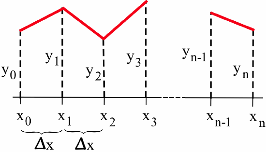
is:\[\left(\Delta x\right)\cdot\left(\frac{y_0+y_1}{2}\right)\nonumber\]Similarly, the areas of the next few trapezoids are:\[\left(\Delta x\right)\cdot\left(\frac{y_1+y_2}{2}\right), \quad \left(\Delta x\right)\cdot\left(\frac{y_2+y_3}{2}\right), \quad \left(\Delta x\right)\cdot\left(\frac{y_3+y_4}{2}\right)\nonumber\]and so on, with the area of the last region being\[\left(\Delta x\right)\cdot\left(\frac{y_{n-1}+y_n}{2}\right)\nonumber\]The sum of these \(n\) trapezoidal areas is:
\begin{align*}
T_n &= \left(\Delta x\right)\left(\frac{y_0+y_1}{2}\right) + \left(\Delta x\right)\left(\frac{y_1+y_2}{2}\right) + \left(\Delta x\right)\left(\frac{y_2+y_3}{2}\right) + \cdots\\
&{\color{white} .} \hspace{7cm} + \left(\Delta x\right)\left(\frac{y_{n-1}+y_n}{2}\right)\\
&= \left(\frac{\Delta x}{2}\right)\left[(y_0+y_1)+(y_1+y_2)+(y_2+y_3)+\cdots +(y_{n-1}+y_n)\right]\\
&= \left(\frac{h}{2}\right)\left[y_0+2y_1 + 2y_2 + 2y_3 + \cdots +2 y_{n-1} + y_n\right]\\
&= \left(\frac{h}{2}\right)\left[f(x_0)+2f(x_1) + 2f(x_2) + 2f(x_3) + \cdots +2 f(x_{n-1}) + f(x_n)\right]\end{align*}
Each \(f\left(x_k\right)\) value, except the first (\(k = 0\)) and the last (\(k = n\)), is the right-endpoint height of one trapezoid and the left-endpoint height of the next, so it shows up in the calculation for two trapezoids and is
multiplied by \(2\) in the formula for the trapezoidal approximation.

Trapezoidal Approximation Rule

If: \(f\) is integrable on \([a,b]\) and \([a,b]\) is partitioned into \(n\) subintervals of width \(h = \frac{b-a}{n}\)

then: the Trapezoidal approximation of \(\displaystyle \int_a^b f(x)\, dx\) is:\[T_n = \frac{h}{2}\left[f(x_0)+2f(x_1) + 2f(x_2) + 2f(x_3) + \cdots +2 f(x_{n-1}) + f(x_n)\right]\nonumber\]

Example \(\PageIndex{1}\)

Compute \(T_4\), the Trapezoidal approximation of \(\displaystyle \int_1^3 f(x)\, dx\) for \(n=4\), with the values of \(f\) in the table below:

\(x\)	\(f(x)\)
1.0	4.2
1.5	3.4
2.0	2.8
2.5	3.6
3.0	3.2

Solution

The step size is \(\displaystyle h = \frac{b-a}{n} = \frac{3-1}{4} = \frac12\) so:
\begin{align*}
T_4 &= \frac{h}{2}\left[f(x_0)+2f(x_1) + 2f(x_2) + 2f(x_3) + f(x_4)\right]\\
&= \frac{0.5}{2} \left[4.2 + 2(3.4) + 2(2.8) + 2(3.6) + (3.2)\right] = (0.25)( 27 ) = 6.75\end{align*}
so we can say that \(\displaystyle \int_1^3 f(x)\, dx \approx 6.75\).

Let’s see how well the Trapezoidal Rule approximates an integral whose value we can compute exactly:\[\int_1^3 x^2\, dx = \frac13 x^3 \bigg|_1^3 = \frac13\left[27-1\right] = \frac{26}{3} \approx 8.6666667\nonumber\]

Example \(\PageIndex{2}\)

Calculate \(T_4\) for \(\displaystyle \int_1^3 x^2\, dx\).

Solution

The step size is \(\displaystyle h = \frac{b-a}{n} = \frac{3-1}{4} = \frac12\) so:
\begin{align*}
T_4 &= \frac{h}{2}\left[f(x_0)+2f(x_1) + 2f(x_2) + 2f(x_3) + f(x_4)\right]\\
&= \frac{0.5}{2} \left[(1.0)^2 + 2(1.5)^2 + 2(2.0)^2 + 2(2.5)^2 + (3.0)^2\right]\\
&= (0.25) \left[1 + 2(2.25) + 2(4) + 2(6.25) + 9\right] =8.75\end{align*}
which is within \(0.1\) of the exact answer. Larger values for \(n\) give better approximations: \(T_{20} = 8.67\) and \(T_{100} = 8.6668\).

Practice \(\PageIndex{1}\)

On a summer day, the level of the pond shown below:

fell 0.1 feet because of evaporation. Use the Trapezoidal Rule to approximate the surface area of the pond and then estimate how much water evaporated.

Answer

Using the Trapezoidal Rule to approximate the pond’s surface area:\[T \approx \frac{5\mbox{ ft}}{2}\cdot\left[\left(0 + 2\cdot 12 + 2 \cdot 14 + 2 \cdot 16 + 2 \cdot 18 + 2\cdot 18 + 0\right)\mbox{ ft}\right] = 390\mbox{ ft}^2\]so the volume is \((\mbox{surface area})(\mbox{depth}) \approx \left(390\mbox{ ft}^2\right)\left(0.1\mbox{ ft}\right) = 39 \mbox{ ft}^3\). FIGURE SOMEWHERE

Approximating a Definite Integral Using Parabolas

If the graph of \(f\) is curved, the slanted lines from the Trapezoidal Rule may not fit the graph of \(f\) as closely as we would like, requiring a large number of subintervals to achieve a good approximation of the definite integral. Curves typically fit the graph of \(f\) better than straight lines in such situations, and the easiest nonlinear curves we know are parabolas.

Note

This parabolic method is known as Simpson’s Rule, named after British mathematician and inventor Thomas Simpson (1710–1761); Germans call it Kepler’sche Fassregel, after Johannes Kepler, who developed it 100 years before Simpson.

Just as we need two points to determine an equation of a line, we will need three points to determine an equation of a parabola.

Calling these points \((x_0, y_0)\), \((x_1, y_1)\) and \((x_2, y_2)\), the area under a parabolic region with evenly spaced \(x_k\) values:

is:\[(2\Delta x)\cdot\left[\frac{y_0+4y_1+y_2}{6}\right] = \frac{\Delta x}{3}\left[y_0+4y_1+y_2\right]\nonumber\](This result is not obvious; see Problem 32 for the necessary algebra.)

Taking the subintervals in pairs, the areas of the next few parabolic regions are:\[\frac{\Delta x}{3}\left[y_2+4y_3+y_4\right], \quad \frac{\Delta x}{3}\left[y_4+4y_5+y_6\right], \quad \frac{\Delta x}{3}\left[y_6+4y_7+y_8\right]\nonumber\]and so on, with the area of the last pair of regions being:\[\frac{\Delta x}{3}\left[y_{n-2}+4y_{n-1}+y_n\right]\nonumber\]so the sum of all \(n\) parabolic areas:

is:
\begin{align*}
S_n &= \frac{\Delta x}{3}\left[y_0+4y_1+y_2\right] + \frac{\Delta x}{3}\left[y_2+4y_3+y_4\right]+\cdots +\frac{\Delta x}{3}\left[y_{n-2}+4y_{n-1}+y_n\right]
&{\color{white} .} \hspace{3cm} + \frac{\Delta x}{3}\left[y_2+4y_3+y_4\right] + \cdots + \frac{\Delta x}{3}\left[y_{n-2}+4y_{n-1}+y_n\right]\\
&= \left(\frac{h}{3}\right)\left[(y_0+4y_1+y_2+y_2+4y_3+y_4 \cdots +y_{n-2}+4y_{n-1}+y_n\right]\\
&= \left(\frac{h}{3}\right)\left[y_0+4y_1 + 2y_2 + 4y_3 + 2y_4+\cdots +2 y_{n-1} + 4y_{n-1} + y_n)\right]\\
&= \left(\frac{h}{3}\right)[f(x_0)+4f(x_1) + 2f(x_2) + 4f(x_3) + 2f(x_4)+\cdots \\
&{\color{white}.} \hspace{5.5cm} +2 f(x_{n-2}) +4 f(x_{n-1}) + f(x_n)]
\end{align*}

In order to use pairs of subintervals, the number \(n\) of subintervals must be even. Notice that the coefficient pattern for the area under a single parabolic region is 1–4–1, but when we put several parabolas next to each other, they share some edges and the pattern becomes 1–4–2–4–2–\(\cdots\)–2–4–1 with the shared edges getting counted twice.

Parabolic Approximation Rule (Simpson’s Rule)

If: \(f\) is integrable on \([a,b]\) and \([a,b]\) is partitioned into \(n\) subintervals of width \(\displaystyle h = \frac{b-a}{n}\)

then: the Parabolic approximation of \(\displaystyle \int_a^b f(x)\, dx\) is:\[S_n = \frac{h}{3}[f(x_0)+4f(x_1) + 2f(x_2) + 4f(x_3) + \cdots + 2 f(x_{n-2}) + 4 f(x_{n-1}) + f(x_n)\nonumber\]

Example \(\PageIndex{3}\)

Calculate \(S_4\), the Simpson’s Rule approximation of \(\displaystyle \int_1^3 f(x)\, dx\) for the function \(f\) with values in this table:

\(x\)	\(f(x)\)
1.0	4.2
1.5	3.4
2.0	2.8
2.5	3.6
3.0	3.2

Solution

The step size is \(\displaystyle h = \frac{b-a}{n} = \frac{3-1}{4} = \frac12\), so:
\begin{align*}S_4 &= \frac{h}{3}\left[f(x_0) + 4f(x_1) + 2f(x_2) + 4f(x_3) + f(x_4)\right]\\
&= \frac{\frac12}{3} \left[4.2 + 4(3.4) + 2(2.8) + 4(3.6) + (3.2)\right] = \frac16 \left( 41 \right) =\frac{41}{6}\end{align*}
or approximately \(6.833\).

Example \(\PageIndex{4}\)

Calculate \(S_4\) for \(\displaystyle \int_1^3 2^x\, dx\).

Solution

As in the previous Examples, \(h = \frac{b-a}{n} = 0.5\) and \(x_0 = 1\), \(x_1 = 1.5\), \(x_2 = 2\), \(x_3 = 2.5\) and \(x_4 = 3\).
\begin{align*}S_4 &= \frac{h}{3}\cdot\left[f(x_0) + 4f(x_1) + 2f(x_2) + 4f(x_3) + f(x_4)\right]\\
&= \frac{\frac12}{3} \cdot\left[f(1) + 4f(1.5) + 2f(2) + 4f(2.5) + f(3)\right]\\
&= \left(\frac16\right) \left[2^1 + 4\left(2^{1.5}\right) + 2\left(2^2\right) + 4\left(2^{2.5}\right) + \left(2^3\right)\right]\\
&= \left(\frac16\right) \left[2 + 4(2\sqrt{2}) + 2(4) + 4(4\sqrt{2}) + 8\right] = \left(\frac16\right)\left[18+20\sqrt{2}\right]\end{align*}
or approximately \(8.656854\). The exact value of the integral is:\[\int_1^3 2^x\, dx = \left[\frac{2^x}{\ln(2)}\right]_1^3 = \frac{8}{\ln(2)}-\frac{2}{\ln(2)} = \frac{6}{\ln(2)} \approx 8.65617024533\nonumber\]Larger values of \(n\) give better approximations: \(S_{20} = 8.656171\) and \(S_{100} = 8.656170\).

Practice \(\PageIndex{2}\)

Use Simpson’s Rule to estimate the surface area of the pond in the figure below:

Answer

Using Simpson’s Rule to approximate the pond's surface area:\[S \approx \frac{5\mbox{ ft}}{3}\cdot\left[\left(0 + 4\cdot 12 + 2 \cdot 14 + 4 \cdot 16 + 2 \cdot 18 + 4\cdot 18 + 0\right)\mbox{ ft}\right] \approx 413\mbox{ ft}^2\]

Which Method Is Best?

The most difficult and time-consuming part of these approximations, whether done by hand or by computer, is the evaluation of the function at the \(x_k\) values. For \(n\) subintervals, all of the methods require about the same number of function evaluations. The table on the next page illustrates how closely each method approximates \(\displaystyle \int_1^5 \frac{1}{x}\, dx = \ln(5) \approx 1.609437912\) using several values of \(n\). The results in the table also show how quickly the actual error shrinks as the value of \(n\) increases: just doubling \(n\) from \(4\) to \(8\) cuts the actual error of the Simpson’s Rule approximation of this definite integral by a factor of \(9\) — a good reward for our extra work.

method	approximation	error bound	actual error
\(T_4\)	1.683333333	0.6666666	0.07389542
\(S_4\)	1.622222222	0.5333333	0.01278431
\(L_4\)	2.083333333	2.0000000	0.47389542
\(R_4\)	1.283333333	2.0000000	0.32610458
\(M_4\)	1.574603175	0.3333333	0.03483474
\(T_8\)	1.628968254	0.1666666	0.01953034
\(S_8\)	1.610846561	0.0333333	0.00140865
\(L_8\)	1.828968254	1.0000000	0.21953034
\(R_8\)	1.428968254	1.0000000	0.18046966
\(M_8\)	1.599844394	0.0833333	0.00959352
\(T_{20}\)	1.612624844	0.0266667	0.00318693
\(S_{20}\)	1.609486789	0.0008533	0.00004888
\(L_{20}\)	1.692624844	0.4000000	0.08318693
\(R_{20}\)	1.532624844	0.4000000	0.07681307
\(M_{20}\)	1.607849324	0.0133333	0.00158859

The “error bounds” in the third column are discussed below. Notice that for each value of \(n\), the Simpson’s Rule approximation \(S_n\) has the smallest error, and that the error for the Midpoint Rule approximation \(M_n\) (discussed in the Problems) is roughly half the error for the Trapezoidal Rule \(T_n\). \(L_n\) and \(R_n\) denote the Left and Right approximations, respectively.

How Good Are the Approximations?

The approximation rules are valuable by themselves, but they are particularly useful because we can find “error bound” formulas that guarantee how close these approximations come to the exact values of the definite integral. It is useful to know that the value of an integral is “about 3.7,” but we can have more confidence in our approximation if we know that value is “within 0.0001 of 3.7.” Then we can decide if our approximation is good enough for the job at hand or if we need to improve it.

We can also solve the formulas for the error bounds provided below to determine how many subintervals we need to guarantee that our approximation is within some specified distance of the exact answer. There is no reason to use 1000 subintervals if 18 will give the needed accuracy. Unfortunately, the formulas for the error bounds require information about the derivatives of the integrands, so we cannot use these error bound formulas for the approximations of integrals of functions defined only by tables or graphs — or of continuous (hence integrable) functions that fail to have continuous derivatives.

The “error bound” formula for the Trapezoidal Rule approximation given at the top of the next page is just a “guarantee”: the actual error is guaranteed to be no larger than the error bound. In fact, the actual error is usually much smaller than the error bound (compare the error bounds with the actual error for \(T_4\), \(T_8\) and \(T_{20}\) in the table above to see this principle in action). The word “error” does not indicate a mistake, it simply means the deviation or distance of the approximate answers from the exact answer.

Error Bound for Trapezoidal Approximation

If: \(f''\) is continuous on \([a,b]\) and \(\left|f''(x)\right|\leq B_2\)

then: the “error” of the \(T_n\) approximation of \(\int_a^b f(x)\, dx\) satisfies:\[\left|\mbox{“error”}\right| = \left|\int_a^b f(x)\, dx - T_n\right|\leq \frac{(b-a)^3 B_2}{12n^2}\nonumber\]

While it’s possible to prove this error bound formula using mathematics you've already learned, the proof is highly technical and sheds little or no insight into the workings of the Trapezoidal Rule, so we (like the authors of most calculus books) have omitted it.

Example \(\PageIndex{5}\)

You can be certain that the \(T_{10}\) approximation of \(\displaystyle \int_0^2 \sin(x^2)\, dx\) is within what distance of the exact value of the integral?

Solution

We know that \(b - a = 2\), \(n = 10\) and \(f(x) = \sin\left(x^2\right)\), so \(f''(x) = -4x^2\cdot\sin\left(x^2\right) + 2\cdot\cos\left(x^2\right)\) is continuous on \([0,2]\). (Practice your differentiation skills by verifying this.)

We now need an “upper bound” for \(\left|f''(x)\right|\). If \(f''(x)\) is differentiable (it is here) then we could use the techniques of Chapter 3 to find its maximum value on \([0,2]\) but that would require finding a third derivative of \(f\), as well as some challenging algebra. Using the triangle inequality and the facts that \(-1 \leq \sin(\theta) \leq 1\) and \(-1 \leq \cos(\theta) \leq 1\), we can conclude:\[\left|f''(x)\right| = \left|-4x^2\cdot\sin\left(x^2\right) + 2\cdot\cos\left(x^2\right)\right| \leq 4x^2\left|sin(x^2)\right|+ 2\left|cos(x^2)\right| \leq 4\cdot2^2\cdot1+2\cdot1 = 18\nonumber\]so we could take \(B_2 = 18\). We can do a bit better, however, by consulting a graph of \(f''(x)\) on \([0,2]\):

it appears clear from the graph that \(\left|f''(x)\right|\leq 11\), so we take \(B_2 = 11\) instead.

Using these values for \(a\), \(b\), \(n\) and \(B_2\) in the “error bound” formula:\[\left|\mbox{“error”}\right| = \left|\int_0^2 \sin(x^2)\, dx - T_{10}\right|\leq \frac{2^3 \cdot 11}{12\cdot{10}^2} = \frac{88}{1200} = \frac{11}{150} < 0.074\nonumber\]so we can be certain that our \(T_{10}\) approximation of the definite integral is within 0.074 of the exact value:\[T_{10} - 0.074 \leq \int_0^2 \sin(x^2)\, dx \leq T_{10} + 0.074\nonumber\]Computing \(T_{10} = 0.7959247\), we can be certain that the value of the integral \(\int_0^2 \sin(x^2)\, dx\) is somewhere between \(0.722\) and \(0.870\).

Note

Notice that (a bound for) the “error” depends on three things: the size of the interval of integration (the bigger the interval, the bigger the potential error); the number of subintervals in the partition (the more subintervals, the smaller the potential error); and the size of the second derivative of the integrand. We've already seen that the second derivative of a function is related to the concavity of its graph — later on we will learn that the second derivative helps measure the “curvature” of the graph of \(f\); it should make sense that the more “curvy” a function is, the less effective a linear approximation technique would be.

Practice \(\PageIndex{3}\)

Find an error bound for the \(T_{12}\) approximation of \(\displaystyle \int_2^5 \frac{1}{x}\, dx\).

Answer

\(b - a = 3\), \(n = 12\) and \(\displaystyle f(x) = \frac{1}{x} \Rightarrow f'(x) = -\frac{1}{x^2} \Rightarrow f''(x) = \frac{2}{x^3}\), so on the interval \([2,5]\):\[\left|f''(x)\right| = \left|\frac{2}{x^3}\right| \leq \frac{2}{2^3} = \frac{1}{4}\]We can therefore take \(B_2 = \frac14\), so:\[\left|\mbox{error}\right| \leq \frac{(b-a)^3\cdot B_2}{12n^2} \leq \frac{3^3\cdot\frac14}{12(12)^2} = \frac{27}{6912} \approx 0.004\]

Example \(\PageIndex{6}\)

How large must \(n\) be to be certain that \(T_n\) is within \(0.001\) of \(\displaystyle \int_0^2 \sin(x^2)\, dx\)?

Solution

Here we know the “allowable error” of \(0.001\) and we must find \(n\). From Example 5 we know that \(b-a=2\) and \(B_2 = 11\), so we want the error bound to be less than the allowable error of \(0.001\): \begin{align*}\frac{2^3 \cdot 11}{12\cdot n^2} < 0.001 \quad &\Rightarrow \quad \frac{12\cdot n^2}{88} > 1000 \quad \Rightarrow \quad n^2 > \frac{88000}{12} \\ &\Rightarrow \quad n > \sqrt{\frac{22000}{3}} \approx 85.6\end{align*} Because \(n\) must be an integer, we can take \(n = 86\). Computing \(T_{86} \approx 0.80465\), we can be certain that the exact value of the integral is between \(0.80365\) and \(0.80565\).

As often happens, \(T_{86}\) is even closer than \(0.001\) to the exact value of the integral:\[\left|T_{86} - \int_0^2 \sin\left(x^2\right)\, dx \right| \approx 0.00012\nonumber\]

Practice \(\PageIndex{4}\)

Determine how large \(n\) must be in order to ensure that \(T_n\) is within \(0.001\) of \(\displaystyle \int_2^5 \frac{1}{x}\, dx\).

Answer

We want:\[\left|\mbox{error}\right| \leq \frac{(b-a)^3\cdot B_2}{12n^2} \leq \frac{3^3\cdot\frac14}{12\cdot n^2} = \frac{27}{48n^2} < 0.001\]so solving for \(n\):\[\frac{48n^2}{27} > 1000 \Rightarrow n^2 > \frac{27000}{48} = \frac{1125}{2} \Rightarrow n > \sqrt{562.5} \approx 23.7\]Using \(n = 24\) will work. We can be certain that \(T_{24}\) is within \(0.001\) of the exact value of the integral. (We cannot guarantee that \(T_{23}\) is within \(0.001\) of the exact value of the integral, but it probably is.)

Error Bound for Simpson’s Parabolic Approximation

If: \(f^{(4)}\) is continuous on \([a,b]\) and \(\left|f^{(4)}(x)\right|\leq B_4\)

then: the “error” of the \(S_n\) approximation of \(\int_a^b f(x)\, dx\) satisfies:\[\left|\mbox{“error”}\right| = \left|\int_a^b f(x)\, dx - S_n\right|\leq \frac{(b-a)^5 B_4}{180n^4}\nonumber\]

Example \(\PageIndex{7}\)

Find an error bound for the \(S_{10}\) approximation of \(\displaystyle\int_0^2 \sin(x^2)\, dx\).

Solution

We have \(b - a = 2\), \(n = 10\) and \(f(x) = \sin(x^2)\), so \(f^{(4)}(x) = (16x^4-12)\sin(x^2) - 48x^2\cos(x^2)\) is continuous on \([0, 2]\). From a graph of \(f^{(4)}(x)\) on \([0, 2]\):

we can estimate that \(B_4 = 165\), so\[\left|\mbox{“error”}\right| = \left|\int_0^2 \sin(x^2)\, dx - S_{10}\right|\leq \frac{2^5 \cdot 165}{180\cdot{10}^4} = \frac{5280}{1800000} < 0.003\nonumber\]and we can be certain that our \(S_{10}\) approximation of \(\int_0^2 \sin(x^2)\, dx\) is within \(0.003\) of the exact value:\[S_{10} - 0.003 \leq \int_0^2 \sin(x^2)\, dx \leq S_{10} + 0.003\nonumber\]Computing \(S_{10} = 0.80537615\), we are certain that the exact value of \(\int_0^2 \sin(x^2)\, dx\) is between \(0.80237615\) and \(0.80837615\). Notice that we achieved a much narrower guarantee using \(S_{10}\) compared to using \(T_{10}\) to approximate the same integral.

Example \(\PageIndex{8}\)

Determine how large \(n\) must be to ensure that \(S_n\) is within \(0.001\) of the exact value of \(\displaystyle \int_0^2 \sin(x^2)\, dx\).

Solution

We want the “error bound” to be less than \(0.001\) and need to find \(n\). We know that \(b-a=2\) and \(B_4 = 165\) \begin{align*}\frac{2^5 \cdot 165}{180\cdot n^4} < 0.001 \quad &\Rightarrow \quad \frac{180\cdot n^2}{5280} > 1000 \quad \Rightarrow \quad n^2 > \frac{5280000}{180} = \frac{88000}{3} \\ &\Rightarrow \quad n > \sqrt[4]{\frac{88000}{3}} \approx 13.09\end{align*} Because \(n\) must be an even integer, we can take \(n = 14\) and be certain that \(S_{14}\) is within \(0.001\) of \(\displaystyle \int_0^2 \sin(x^2)\, dx\).

As we have come to expect, \(S_{14}\) is even closer than \(0.001\) to the exact value of the integral; using advanced methods, we can show that:\[\left|\int_0^2 \sin(x^2)\, dx - S_{14}\right| \approx 0.00015\nonumber\]

Alternative Methods

In Section 8.7 and in Chapter 10, you will learn how to approximate a function \(f\) over an entire interval \([a,b]\) using a single polynomial \(p(x)\) of degree \(n\); you can then approximate \(\int_a^b f(x)\, dx\) with \(\int_a^b p(x)\, dx\), which is relatively easy to compute. One advantage of this method is that (once we have found \(p(x)\)), we only need to evaluate another polynomial (\(P(x)\) where \(P'(x)=p(x)\)) at two values (\(P(a)\) and \(P(b)\)) to compute \(\int_a^b p(x)\, dx \approx \int_a^b f(x)\, dx\) and we can get better approximations by increasing \(n\) and using polynomials of higher and higher degree; using the Trapezoidal Rule or Simpson’s Rule requires us to evaluate \(f(x)\) at \(n+1\) points. A disadvantage of this approach is that our original \(f(x)\) must have \(n\) continuous derivatives, which is not always the case, and we need to be able to compute those \(n\) derivatives at a single point. Most textbooks on Numerical Analysis offer more sophisticated techniques for approximating definite integrals.

Using Technology

If you have written even the most basic computer code, you should be able to write a program to compute any Trapezoidal Rule or Simpson’s Rule approximation you want (accurate up to the floating-point limitations of the machine running your code). If you have a graphing calculator, it likely has one or more numerical integration utilities:

The Web site Wolfram|Alpha (www.wolframalpha.com) can approximate definite integrals to any desired accuracy; typing integral sin(x^2) from x=0 to x=2 yields:

Wolfram|Alpha can also be used to quickly apply Simpson’s Rule: use Simpson's rule sin(x^2) from 0 to 2 with 10 intervalsyields an approximation of \(0.804811\) for \(\int_0^2 \sin(x^2)\, dx\).

Problems

1. Use the values in the table below to approximate \(\int_2^6 f(x)\, dx\) by calculating \(T_4\) and \(S_4\).

   \(x\)	\(f(x)\)
   2.0	2.1
   2.5	2.7
   3.0	3.8
   3.5	2.3
   4.0	0.3
   4.5	-1.8
   5.0	-0.9
   5.5	0.5
   6.0	2.2

2. Use the values in the table above to approximate \(\int_2^6 f(x)\, dx\) by calculating \(T_8\) and \(S_8\).
3. Use the values in the table below to approximate \(\int_{-3}^1 g(x)\, dx\) by calculating \(T_8\) and \(S_8\).

   \(x\)	\(g(x)\)
   -3.0	4.2
   -2.5	1.8
   -2.0	0.7
   -1.5	1.5
   -1.0	3.4
   -0.5	4.3
   0.0	3.5
   0.5	-0.3
   1.0	-4.6

4. Use the values in the table above to approximate \(\int_{-3}^1 g(x)\, dx\) by calculating \(T_4\) and \(S_4\).

For Problems 5–10, calculate:

1. \(T_4\)
2. \(S_4\)
3. the exact value of the integral.

5. \(\displaystyle \int_1^3 x \, dx\)
6. \(\displaystyle \int_0^2 \left[1-x\right] \, dx\)
7. \(\displaystyle \int_{-1}^1 x^2 \, dx\)
8. \(\displaystyle \int_2^6 \frac{1}{x} \, dx\)
9. \(\displaystyle \int_0^{\pi} \sin(x) \, dx\)
10. \(\displaystyle \int_0^1 \sqrt{x} \, dx\)

For Problems 11–16, calculate:

1. \(T_6\)
2. \(S_6\)

11. \(\displaystyle \int_0^2 \frac{1}{1+x^3} \, dx\)
12. \(\displaystyle \int_1^2 2^x \, dx\)
13. \(\displaystyle \int_{-1}^1 \sqrt{4-x^2} \, dx\)
14. \(\displaystyle \int_0^1 e^{-x^2} \, dx\)
15. \(\displaystyle \int_1^4 \frac{\sin(x)}{x} \, dx\)
16. \(\displaystyle \int_0^1 \sqrt{1+\sin(x)} \, dx\)

For Problems 17–22, calculate:

1. the error bound for \(T_4\)
2. the error bound for \(S_4\)
3. the value of \(n\) so that the error bound for \(T_n\) is less than \(0.001\)
4. the value of \(n\) so that the error bound for \(S_n\) is less than \(0.001\).

17. \(\displaystyle \int_1^3 x \, dx\)
18. \(\displaystyle \int_0^2 \left[1-x\right] \, dx\)
19. \(\displaystyle \int_{-1}^1 x^3 \, dx\)
20. \(\displaystyle \int_2^6 \frac{1}{x} \, dx\)
21. \(\displaystyle \int_0^{\pi} \sin(x) \, dx\)
22. \(\displaystyle \int_0^1 \sqrt{x} \, dx\)
23. Estimate the area of the piece of land located between the river and the road in the figure below:
    
24. Estimate the area of the island in the figure below:
    
25. Estimate the volume of water in the reservoir shown below if the average depth is 22 feet:
    
26. The table below shows the speedometer readings (in feet per minute) for a car at one-minute intervals:

    \(t\)	\(v(t)\)	\(t\)	\(v(t)\)
    0	0	6	5200
    1	2000	7	4400
    2	3000	8	3000
    3	5000	9	2000
    4	5000	10	1200
    5	6000

    Estimate how far the car traveled:
    1. during the first 5 minutes of the trip and
    2. during the first 10 minutes of the trip.
27. The table below shows the speed (in feet per minute) of a jogger at one-minute intervals:

    \(t\)	\(v(t)\)	\(t\)	\(v(t)\)
    0	0	6	520
    1	420	7	440
    2	540	8	360
    3	300	9	260
    4	500	10	180
    5	580

    Estimate how far the jogger ran during her workout.
28. Use the error-bound formula for Simpson’s Rule to show that the parabolic approximation gives the exact value of \(\int_a^b f(x)\, dx\) if \(f(x) = Ax^3 + Bx^2 + Cx + D\) is a polynomial of degree 3 or less.
29. A trapezoidal region with base \(b\) and heights \(h_1\) and \(h_2\) (assume \(h_1 \neq h_2\)) can be cut into a rectangle with base \(b\) and height \(h_1\) and a triangle with base \(b\) and height \(h_1 - h_2\):
    
    Show that the sum of the area of the rectangle and the area of the triangle is \(\displaystyle b\cdot\left[\frac{h_1 + h_2}{2}\right]\).
30. Let \(f(m)\) be the minimum value of \(f\) on the interval \([x_0, x_1]\), \(f(M)\) be the maximum value of \(f\) on \([x_0, x_1]\), and \(h = x_1 - x_0\). Show that:\[h\cdot f(m) \leq b\cdot\left[\frac{f(x_0) + f(x_1}{2}\right] \leq h\cdot f(M)\nonumber\]and use this result to show that the trapezoidal approximation is between the lower and upper Riemann sums for \(f\). Because the limit (as \(h\rightarrow 0\)) of these Riemann sums is \(\int_a^b f(x)\, dx\), conclude that the limit of the trapezoidal sums must equal \(\int_a^b f(x)\, dx\).
31. Let \(f(m)\) be the minimum value of \(f\) on the interval \([x_0, x_2]\), \(f(M)\) the maximum of \(f\) on \([x_0, x_2]\) and \(h = x_1 - x_0 = x_2 - x_1\). Show that the value\[2h\cdot\left[\frac{f(x_0) + 4f(x_1) + f(x_2)}{6}\right]\nonumber\]is between \(2h\cdot f(m)\) and \(2h\cdot f(M)\) and use this result to show that the parabolic approximation of \(\int_a^b f(x) \, dx\) is between the lower and upper Riemann sums for \(f\). Conclude that the limit of the parabolic sums must equal \(\int_a^b f(x)\, dx\).
32. This problem guides you through the steps to show that the area under a parabolic region with evenly spaced \(x_k\) values:
    
    (which, for the purposes of this problem we will call \(x_0 = m-h\), \(x_1 = m\) and \(x_2 = m+h\)) is:\[\frac{h}{3}\cdot \left[f(x_0) + 4f(x_1) + f(x_2)\right] = \frac{h}{3}\cdot \left[y_0 + 4y_1 + y_2\right]\nonumber\]
    1. For \(f(x) = Ax^2 + Bx + C\), verify that:\[\int_{m-h}^{m+h} f(x)\, dx = \frac{A}{3}x^3 + \frac{B}{2}x^2+Cx\big|_{m-h}^{m+h} = 2Am^2h + \frac23 A h^3 + 2Bmh+2Ch\nonumber\]
    2. Expand each of the polynomials: \begin{align*} y_0 = f(m-h) &= A(m-h)^2 + B(m-h) + C\\ y_1 = f(m) &= Am^2 + Bm + C\\ y_2 = f(m+h) &= A(m+h)^2 + B(m+h) + C\end{align*} and use the results to verify that: \begin{align*} \frac{h}{3}\left[y_0+4y_1 + y_2\right] &= 2h\left[\frac{f(m-h) +4f(m)+f(m+h)}{6}\right]\\ &= 2Am^2h + \frac23 A h^3 + 2Bmh+2Ch\end{align*}
    3. Compare the results of parts (a) and (b) to conclude that for any quadratic function \(f(x) = Ax^2 + Bx + C\):\[\int_{m-h}^{m+h} f(x)\, dx =\frac{h}{3}\left[y_0 + 4y_1 + y_2\right]\nonumber\]

Left-Endpoint, Right-Endpoint and Midpoint Rules

The rectangular approximation methods approximate an integrand with horizontal lines, so that the approximating regions are rectangles and the sum of the areas of these rectangular regions is a Riemann sum. The Left- and Right-Endpoint Rules are easy to understand and use, but they typically require a very large number of subintervals to ensure good approximations of a definite integral. The Midpoint Rule uses the value of the integrand at the midpoint of each subinterval: if these midpoint values of \(f\) are available (for example, when \(f\) is given by a formula) then the Midpoint Rule is often more efficient than the Trapezoidal rule. The rectangular approximation rules are: \begin{align*} L_n &= h\cdot\left[f(x_0) + f(x_1) + f(x_2) + \cdots + f(x_{n-1})\right]\\ R_n &= h\cdot\left[f(x_1) + f(x_2) + f(x_3) + \cdots + f(x_n)\right]\\ M_n &= h\cdot\left[f(c) + f(c + h) + f(c + 2h) + \cdots + f(c + (n-1)h)\right] \end{align*} where \(\displaystyle c = x_0 + \frac{h}{2}\) so that the points \(c\), \(c + h\), \(c + 2h\), etc. are the midpoints of the subintervals. The “error bounds” for these methods are: \begin{align*} \left|\mbox{“error” for }L_n\mbox{ or }R_n\right| &\leq \frac{(b-a)^2 B_1}{2n}\\ \left|\mbox{“error” for }M_n\right| &\leq \frac{(b-a)^3 B_2}{24n^2} \end{align*} where \(B_1 \geq \left|f'(x)\right|\) on \([a,b]\) and \(B_2 \geq \left|f''(x)\right|\) on \([a,b]\). Notice that the error bound for \(M_n\) is half the error bound of \(T_n\), the trapezoidal approximation.

For Problems 33–38, calculate:

1. \(L_4\)
2. \(R_4\)
3. \(M_4\)
4. the exact value of the integral.

33. \(\displaystyle \int_1^3 x \, dx\)
34. \(\displaystyle \int_0^2 \left[1-x\right] \, dx\)
35. \(\displaystyle \int_{-1}^1 x^2 \, dx\)
36. \(\displaystyle \int_2^6 \frac{1}{x} \, dx\)
37. \(\displaystyle \int_0^{\pi} \sin(x) \, dx\)
38. \(\displaystyle \int_0^1 \sqrt{x} \, dx\)
39. Show that the Trapezoidal approximation is the average of the Left- and Right-Endpoint approximations: \(\displaystyle T_n = \frac12\left(L_n + R_n\right)\).

The integrals in Problems 40–43 will arise in applications from Chapter 5. Use technology to approximate each integral by applying Simpson’s Rule with \(n = 10\) and \(n = 40\) to approximate their values. (Is \(S_{40}\) very different from \(S_{10}\)?)

40. \(\displaystyle \frac{1}{\sqrt{2\pi}} \int_{-2}^{2} e^{-\frac12 x^2}\, dx\)
41. \(\displaystyle \int_{-1}^{2} \sqrt{1+4x^2}\, dx\)
42. \(\displaystyle \int_{0}^{\pi} \sqrt{1+\cos^2(x)}\, dx\)
43. \(\displaystyle \int_{0}^{2\pi} \sqrt{16\sin^2(t)+9\cos^2(t)}\, dt\)