2.2: Differentials and Tangent Lines

Suppose we are given a curve \(y = f(x)\) and at a point \((a, b)\) on the curve the slope \(f'(a)\) is defined. Then the tangent line to the curve at the point \((a, b)\), illustrated in Figure \(\PageIndex{1}\), is defined to be the straight line which passes through the point \((a, b)\) and has the same slope as the curve at \(x = a\). Thus the tangent line is given by the equation \[l(x) - b = f'(a) (x-a), \nonumber\] or \[l(x) = f'(a)(x - a) + b. \nonumber\]

Figure \(\PageIndex{1}\): Tangent lines.

Example \(\PageIndex{1}\)

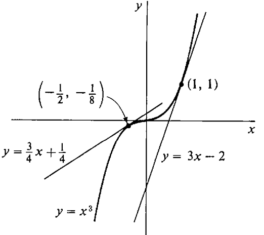
For the curve \(y = x^{3}\), find the tangent lines at the points \((0, 0)\), \((1, 1)\), and \((-\frac{1}{2}, -\frac{1}{8}\) (Figure \(\PageIndex{2}\)).

Figure \(\PageIndex{2}\): Tangent lines to points on the curve \(y = x^{3}\).

Solution

The slope is given by \(f'(x) = 3x^{2}\). At \(x = 0\), \(f'(0) = 3 \cdot 0^{2} = 0\). The tangent line has the equation \[y = 0(x - 0) + 0, \quad \text{or} \quad y = 0. \nonumber\]

At \(x = 1\), \(f'(1) = 3\), whence the tangent line is \[y = 3(x - 1) + 1, \quad \text{or} \quad y = 3x - 2. \nonumber\]

At \(x = -\frac{1}{2}\), \(f'(-\frac{1}{2}) = 3 \cdot (-\frac{1}{2})^{2} = \frac{3}{4}\) so the tangent line is \[y = \frac{3}{4} \left(x - \left(-\frac{1}{2}\right)\right) + \left(-\frac{1}{8}\right), \quad \text{or } y = \frac{3}{4}x + \frac{1}{4}. \nonumber\]

Given a curve \(y = f(x)\), suppose that \(x\) starts out with the value \(a\) and then changes by an infinitesimal amount \(\Delta x\). What happens to \(y\)? Along the curve, \(y\) will change by the amount \[f(a + \Delta x) - f(a) = \Delta y. \nonumber\]

But along the tangent line \(y\) will change by the amount \[\begin{align*} l(a + \Delta x) - l(a) &= [f'(a) (a + \Delta x - a) + b] - [f'(a) (a-a) + b] \\ &= f'(a) \Delta x. \end{align*}\]

When \(x\) changes from \(a\) to \(a + \Delta x\), we see that: \[\begin{align*} \text{change in } y \text{ along curve} &= f(a + \Delta x) - f(a), \\ \text{change in } y \text{ along tangent line} &= f'(a) \Delta x. \end{align*}\]

In the last section we introduced the dependent variable \(\Delta y\), the increment of \(y\), with the equation \[\Delta y = f(x + \Delta x) - f(x). \nonumber\]\(\Delta y\) is equal to the change in \(y\) along the curve as \(x\) changes to \(x + \Delta x\).

The following theorem gives a simple but useful formula for the increment \(\Delta y\).

Increment Theorem

Let \(y = f(x)\). Suppose \(f'(x)\) exists at a certain point \(x\), and \(\Delta x\) is ifinitesimal. Then \(\Delta y\) is infinitesimal, and \[\Delta y = f'(x) \Delta x + \varepsilon \Delta x \nonumber\]for some infinitesimal \(\varepsilon\), which depends on \(x\) and \(\Delta x\).

Proof

Case 1: \(\Delta x = 0\).

In this case, \(\Delta y = f'(x) \Delta x = 0\), and we put \(\varepsilon = 0\).

Case 2: \(\Delta x \neq 0\).

In this case, \[\frac{\Delta y}{\Delta x} \approx f'(x); \nonumber\]

so for some infinitesimal \(\varepsilon\), \[\frac{\Delta y}{\Delta x} = f'(x) + \varepsilon. \nonumber\]

Multiplying both sides by \(\Delta x\), \[\Delta y = f'(x) \Delta x + \varepsilon \Delta x. \nonumber\]

Example \(\PageIndex{2}\)

Let \(y = x^{3}\), so that \(y' = 3x^{2}\). According to the Increment Theorem, \[\Delta y = 3x^{2} \Delta x + \varepsilon \Delta x \nonumber\]for some infinitesimal \(\varepsilon\). Find \(\varepsilon\) in terms of \(x\) and \(\Delta x\) when \(\Delta x \neq 0\).

Solution

We have \[\begin{align*} \Delta y &= 3x^{2} \Delta x + \varepsilon \Delta x, \frac{\Delta y}{\Delta x} = 3x^{2} + \varepsilon, \\ \varepsilon &= \frac{\Delta y}{\Delta x} - 3x^{2}. \end{align*}\]

We must still eliminate \(\Delta y\). From Example \(2.1.1\), \[\begin{align*} \Delta y = (x + \Delta x)^{3} - x^{3}, \\ \frac{\Delta y}{\Delta x} &= 3x^{2} + 3x \Delta x + (\Delta x)^{2}. \end{align*}\]

Substituting, \[\varepsilon = \left(3x^{2} + 3x \Delta x + (\Delta x)^{2}\right) - 3x^{2}. \nonumber\]

Since \(3x^{2}\) cancels, \[\varepsilon = 3x \Delta x + (\Delta x)^{2}. \nonumber\]

We shall now introduce a new dependent variable \(dy\), called the differential of \(y\), with the equation \[dy = f'(x) \Delta x. \nonumber\]

\(dy\) is equal to the change in \(y\) along the tangent line as \(x\) changes to \(x + \Delta x\). In Figure \(\PageIndex{3}\) we see \(dy\) and \(\Delta y\) under the microscope.

Figure \(\PageIndex{3}\): \(\Delta y = \text{change in } y \text{ along curve}\)
\(dy = \text{change in } y \text{ along tangent line}\)

To keep our notation uniform we also introduce the symbol \(dx\) as another name for \(\Delta x\). For an independent variable \(x\), \(\Delta x\) and \(dx\) are the same, but for a dependent variable \(y\), \(\Delta y\) and \(dy\) are different.

Definition:

Suppose \(y\) depends on \(x\), \(y = f(x)\).

(i) The differential of \(x\) is the independent variable \(dx = \Delta x\).
(ii) The differential of \(y\) is the dependent variable \(dy\) given by \[dy = f'(x) \ dx. \nonumber\]When \(dx \neq 0\), the equation above may be rewritten as \[\frac{dy}{dx} = f'(x). \nonumber\]

Compare this equation with \[\frac{\Delta y}{\Delta x} \approx f'(x). \nonumber\]

The quotient \(dy/dx\) is a very convenient alternative symbol for the derivative \(f'(x)\). In fact we shall write the derivative in the form \(dy/dx\) most of the time.

The differential \(dy\) depends on two independent variables \(x\) and \(dx\). In functional notation, \[dy = df(x, dx) \nonumber\]where \(df\) is the real function of two variables defined by \[df(x, dx) = f'(x) dx. \nonumber\]

When \(dx\) is substituted for \(\Delta x\) and \(dy\) for \(f'(x) dx\), the Increment Theorem takes the short form \[\Delta y = dy + \varepsilon \ dx. \nonumber\]

The Increment Theorem can be explained graphically using an infinitesimal microscope. Under an infinitesimal microscope, a line of length \(\Delta x\) is magnified to a line
of unit length, but a line of length \(\varepsilon \Delta x\) is only magnified to an infinitesimal length \(\varepsilon\). Thus the Increment Theorem shows that when \(f'(x)\) exists:

1. The differential \(dy\) and the increment \(\Delta y = dy + e \ dx\) are so close to each other that they cannot be distinguished under an infinitesimal microscope.
2. The curve \(y = f(x)\) and the tangent line at \((x, y)\) are so close to each other that they cannot be distinguished under an infinitesimal microscope; both look like a straight line of slope \(f'(x)\).

Figure \(\PageIndex{3}\) is not really accurate. The curvature had to be exaggerated in order to distinguish the curve and tangent line under the microscope. To give an accurate picture, we need a more complicated figure like Figure \(\PageIndex{4}\), which has a second infinitesimal microscope trained on the point \((a + \Delta x, b + \Delta y)\) in the field of view of the original microscope. This second microscope magnifies \(\varepsilon \ dx\) to a unit length and magnifies \(\Delta x\) to an infinite length.

Figure \(\PageIndex{4}\): Magnified view of the separation between curve and tangent line.

Example \(\PageIndex{3}\)

Whenever a derivative \(f'(x)\) is known, we can find the differential \(dy\) at once by simply multiplying the derivative by \(dx\), using the formula \(dy = f'(x) \ dx\). The examples in the last section give the following differentials.

\(\begin{aligned} &\text{(a)} \ y = x^{3}, \quad\quad\quad\quad &&dy = 3x^{2} dx \\ &\text{(b)} \ y = \sqrt{x}, &&dy = \dfrac{dx}{2 \sqrt{x}} \text{ where } x>0 \\ &\text{(c)} \ y = 1/x, &&dy = -dx/x^{2} \ \text{ when } x \neq 0 \\ &\text{(d)} \ y = |x|, &&dy = \begin{cases} dx \ & \text{when } x > 0, \\ -dx &\text{when } x < 0, \\ \text{undefined} & \text{when } x=0. \end{cases} \\ &\text{(e)} \ y = bt - 16t^{2}, &&dy = (b-32t) \ dt. \end{aligned}\)

The differential notation may also be used when we are given a system of formulas in which two or more dependent variables depend on an independent variable. For example if \(y\) and \(z\) are functions of \(x\), \[y = f(x), \quad z = g(x), \nonumber\]then \(\Delta y\), \(\Delta z\), \(dy\), \(dz\) are determined by \[\begin{align*} & \Delta y = f(x + \Delta x) - f(x), \quad\quad\quad && \Delta z = g(x + \Delta x) - g(x), \\ & dy = f'(x)dx, && dz = g'(x) dx. \end{align*}\]

Example \(\PageIndex{4}\)

Given \(y = \frac{1}{2}x\), \(z = x^{3}\), with \(x\) as the independent variable, then \[\begin{align*} \Delta y &= \frac{1}{2} (x + \Delta x) - \frac{1}{2} x = \frac{1}{2} x, \\ \Delta z &= 3x^{2} \Delta x + 3x (\Delta x)^{2} + (\Delta x)^{3}, \\ dy &= \frac{1}{2} dx, \quad dz = 3x^{2} dx \end{align*}\]

The meaning of the symbols for increment and differential in this example will be different if we take \(y\) as the independent variable. Then \(x\) and \(z\) are functions of \(y\). \[x = 2y, \quad z = 8y^{3} \nonumber\]

Now \(\Delta y = dy\) is just an independent variable, while \[\begin{align*} \Delta x &= 2(y + \Delta y) - 2y = 2 \Delta y, \\ \Delta z &= 8(y + \Delta y)^{3} \\ &= 8 \left[3y^{2} \Delta y + 3y (\Delta y)^{2} + (\Delta y)^{3}\right] \\ &= 24y^{2} \Delta y + 24y(\Delta y)^{2} + 8(\Delta y)^{3}. \end{align*}\]

Moreover, \[dx = 2 \ dy, \quad dz = 24y^{2} \ dy. \nonumber\] 

We may also apply the differential notation to terms. If \(\tau(x)\) is a term with the variable \(x\), then \(\tau(x)\) determines a function \(f\), \[\tau(x) = f(x), \nonumber\]

and the differential \(d(\tau(x))\) has the meaning \[d(\tau(x)) = f'(x) \ dx. \nonumber\]

Example \(\PageIndex{5}\)

\(\begin{aligned} &\text{(a)} \ &&d\left(x^{3}\right) = 3x^{2} \ dx. \\ &\text{(b)} &&d(\sqrt{x}) = \dfrac{dx}{2 \sqrt{x}}, \quad x>0 \\ &\text{(c)} &&d(1/x) = -\frac{dx}{x^{2}}, \quad x \neq 0. \\ &\text{(d)} &&d(|x|) = \begin{cases} dx & \text{when } x>0, \\ -dx & \text{when } x<0, \\ \text{undefined} & \text{when } x=0. \end{cases} \\ &\text{(e)} \ &\text{Let } u = bt \text{ and } w=-16t^{2}. \text{ Then} \end{aligned}\)

\[u + w = bt - 16t^{2}, \quad d(u+w) = (b-32t) dt. \nonumber\] 

Problems for Section 2.2

In Problems 1-8, express \(\Delta y\) and \(dy\) as functions of \(x\) and \(\Delta x\), and for \(\Delta x\) infinitesimal find an infinitesimal \(\varepsilon\) such that \(\Delta y = dy + \varepsilon \Delta x\).

1.	\(y = x^{2}\)	2.	\(y = -5x^{2}\)
3.	\(y = 2\sqrt{x}\)	4.	\(y = x^{4}\)
5.	\(y = 1/x\)	6.	\(y = x^{-2}\)
7.	\(y = x - 1/x\)	8.	\(y = 4x + x^{3}\)
9.	If \(y = 2x^{2}\) and \(z = x^{3}\), find \(\Delta y\), \(\Delta z\), \(dy\), and \(dz\).
10.	If \(y = 1/(x + 1)\) and \(z = 1/(x + 2)\), find \(\Delta y\), \(\Delta z\), \(dy\), and \(dz\).
11.	Find \(d(2x+1)\).	12.	Find \(d\left(x^{2} - 3x)\).
13.	Find \(d\sqrt{x + 1}\).	14.	Find \(d(\sqrt{2x + 1})\).
15.	Find \(d(ax + b)\).	16.	Find \(d(ax^{2})\).
17.	Find \(d(3 + 2/x)\).	18.	Find \(d(x \sqrt{x})\).
19.	Find \(d(1/\sqrt{x}\).	20.	Find \(d \left(x^{3} - x^{2}\).
21.	Let \(y = \sqrt{x}\), \(z = 3x\). Find \(d(y + z)\) and \(d(y/z)\).
22.	Let \(y = x^{-1}\) and \(z = x^{3}\). Find \(d(y + z)\) and \(d(y/z)\).

In Problems 23-30 below, find the equation of the line tangent to the given curve at the given point.

23.	\(y = x^{2}; (2,4)\)	24.	\(y = 2x^{2}; (-1,2)\)
25.	\(y = -x^{2}; (0,0)\)	26.	\(y = \sqrt{x}; (1,1)\)
27.	\(y = 3x-4; (1, -1)\)	28.	\(y = \sqrt{t-1}; (5, 2)\)
29.	\(y = x^{4}; (-2, 16)\)	30.	\(y = x^{3} - x; (0, 0)\)
31.	Find the equation of the line tangent to the parabola \(y = x^{2}\) at the point \(\left(x_{0}, x_{0}^{2}\right)\).
32.	Find all points P\(\left(x_{0}, x_{0}^{2}\right)\) on the parabola \(y = x^{2}\) such that the tangent line at \(P\) passes through the point \((0, -4)\).
\(\square\) 33.	Prove that the line tangent to the parabola \(y = x^{2}\) at P\(\left(x_{0}, x_{0}^{2}\right)\) does not meet the parabola at any point except \(P\).