
1.7: Slope of a Line and Graphing Lines
- Page ID
- 193574

\( \newcommand{\vecs}[1]{\overset { \scriptstyle \rightharpoonup} {\mathbf{#1}} } \)
\( \newcommand{\vecd}[1]{\overset{-\!-\!\rightharpoonup}{\vphantom{a}\smash {#1}}} \)
\( \newcommand{\dsum}{\displaystyle\sum\limits} \)
\( \newcommand{\dint}{\displaystyle\int\limits} \)
\( \newcommand{\dlim}{\displaystyle\lim\limits} \)
\( \newcommand{\id}{\mathrm{id}}\) \( \newcommand{\Span}{\mathrm{span}}\)
( \newcommand{\kernel}{\mathrm{null}\,}\) \( \newcommand{\range}{\mathrm{range}\,}\)
\( \newcommand{\RealPart}{\mathrm{Re}}\) \( \newcommand{\ImaginaryPart}{\mathrm{Im}}\)
\( \newcommand{\Argument}{\mathrm{Arg}}\) \( \newcommand{\norm}[1]{\| #1 \|}\)
\( \newcommand{\inner}[2]{\langle #1, #2 \rangle}\)
\( \newcommand{\Span}{\mathrm{span}}\)
\( \newcommand{\id}{\mathrm{id}}\)
\( \newcommand{\Span}{\mathrm{span}}\)
\( \newcommand{\kernel}{\mathrm{null}\,}\)
\( \newcommand{\range}{\mathrm{range}\,}\)
\( \newcommand{\RealPart}{\mathrm{Re}}\)
\( \newcommand{\ImaginaryPart}{\mathrm{Im}}\)
\( \newcommand{\Argument}{\mathrm{Arg}}\)
\( \newcommand{\norm}[1]{\| #1 \|}\)
\( \newcommand{\inner}[2]{\langle #1, #2 \rangle}\)
\( \newcommand{\Span}{\mathrm{span}}\) \( \newcommand{\AA}{\unicode[.8,0]{x212B}}\)
\( \newcommand{\vectorA}[1]{\vec{#1}} % arrow\)
\( \newcommand{\vectorAt}[1]{\vec{\text{#1}}} % arrow\)
\( \newcommand{\vectorB}[1]{\overset { \scriptstyle \rightharpoonup} {\mathbf{#1}} } \)
\( \newcommand{\vectorC}[1]{\textbf{#1}} \)
\( \newcommand{\vectorD}[1]{\overrightarrow{#1}} \)
\( \newcommand{\vectorDt}[1]{\overrightarrow{\text{#1}}} \)
\( \newcommand{\vectE}[1]{\overset{-\!-\!\rightharpoonup}{\vphantom{a}\smash{\mathbf {#1}}}} \)
\( \newcommand{\vecs}[1]{\overset { \scriptstyle \rightharpoonup} {\mathbf{#1}} } \)
\(\newcommand{\longvect}{\overrightarrow}\)
\( \newcommand{\vecd}[1]{\overset{-\!-\!\rightharpoonup}{\vphantom{a}\smash {#1}}} \)
\(\newcommand{\avec}{\mathbf a}\) \(\newcommand{\bvec}{\mathbf b}\) \(\newcommand{\cvec}{\mathbf c}\) \(\newcommand{\dvec}{\mathbf d}\) \(\newcommand{\dtil}{\widetilde{\mathbf d}}\) \(\newcommand{\evec}{\mathbf e}\) \(\newcommand{\fvec}{\mathbf f}\) \(\newcommand{\nvec}{\mathbf n}\) \(\newcommand{\pvec}{\mathbf p}\) \(\newcommand{\qvec}{\mathbf q}\) \(\newcommand{\svec}{\mathbf s}\) \(\newcommand{\tvec}{\mathbf t}\) \(\newcommand{\uvec}{\mathbf u}\) \(\newcommand{\vvec}{\mathbf v}\) \(\newcommand{\wvec}{\mathbf w}\) \(\newcommand{\xvec}{\mathbf x}\) \(\newcommand{\yvec}{\mathbf y}\) \(\newcommand{\zvec}{\mathbf z}\) \(\newcommand{\rvec}{\mathbf r}\) \(\newcommand{\mvec}{\mathbf m}\) \(\newcommand{\zerovec}{\mathbf 0}\) \(\newcommand{\onevec}{\mathbf 1}\) \(\newcommand{\real}{\mathbb R}\) \(\newcommand{\twovec}[2]{\left[\begin{array}{r}#1 \\ #2 \end{array}\right]}\) \(\newcommand{\ctwovec}[2]{\left[\begin{array}{c}#1 \\ #2 \end{array}\right]}\) \(\newcommand{\threevec}[3]{\left[\begin{array}{r}#1 \\ #2 \\ #3 \end{array}\right]}\) \(\newcommand{\cthreevec}[3]{\left[\begin{array}{c}#1 \\ #2 \\ #3 \end{array}\right]}\) \(\newcommand{\fourvec}[4]{\left[\begin{array}{r}#1 \\ #2 \\ #3 \\ #4 \end{array}\right]}\) \(\newcommand{\cfourvec}[4]{\left[\begin{array}{c}#1 \\ #2 \\ #3 \\ #4 \end{array}\right]}\) \(\newcommand{\fivevec}[5]{\left[\begin{array}{r}#1 \\ #2 \\ #3 \\ #4 \\ #5 \\ \end{array}\right]}\) \(\newcommand{\cfivevec}[5]{\left[\begin{array}{c}#1 \\ #2 \\ #3 \\ #4 \\ #5 \\ \end{array}\right]}\) \(\newcommand{\mattwo}[4]{\left[\begin{array}{rr}#1 \amp #2 \\ #3 \amp #4 \\ \end{array}\right]}\) \(\newcommand{\laspan}[1]{\text{Span}\{#1\}}\) \(\newcommand{\bcal}{\cal B}\) \(\newcommand{\ccal}{\cal C}\) \(\newcommand{\scal}{\cal S}\) \(\newcommand{\wcal}{\cal W}\) \(\newcommand{\ecal}{\cal E}\) \(\newcommand{\coords}[2]{\left\{#1\right\}_{#2}}\) \(\newcommand{\gray}[1]{\color{gray}{#1}}\) \(\newcommand{\lgray}[1]{\color{lightgray}{#1}}\) \(\newcommand{\rank}{\operatorname{rank}}\) \(\newcommand{\row}{\text{Row}}\) \(\newcommand{\col}{\text{Col}}\) \(\renewcommand{\row}{\text{Row}}\) \(\newcommand{\nul}{\text{Nul}}\) \(\newcommand{\var}{\text{Var}}\) \(\newcommand{\corr}{\text{corr}}\) \(\newcommand{\len}[1]{\left|#1\right|}\) \(\newcommand{\bbar}{\overline{\bvec}}\) \(\newcommand{\bhat}{\widehat{\bvec}}\) \(\newcommand{\bperp}{\bvec^\perp}\) \(\newcommand{\xhat}{\widehat{\xvec}}\) \(\newcommand{\vhat}{\widehat{\vvec}}\) \(\newcommand{\uhat}{\widehat{\uvec}}\) \(\newcommand{\what}{\widehat{\wvec}}\) \(\newcommand{\Sighat}{\widehat{\Sigma}}\) \(\newcommand{\lt}{<}\) \(\newcommand{\gt}{>}\) \(\newcommand{\amp}{&}\) \(\definecolor{fillinmathshade}{gray}{0.9}\)By the end of this section, you will be able to:
- Find the slope of a line
- Graph a line given a point and the slope
- Graph a line using its slope and intercept
- Graph a line given the intercepts
- Choose the most convenient method to graph a line
- Graph and interpret applications of slope–intercept
- Use slopes to identify parallel and perpendicular lines
Find the Slope of a Line
When you graph linear equations, you may notice that some lines rise up as they go from left to right and some lines decline. Some lines are very steep and some lines are more flatter mathematics, the measure of the steepness of a line is called the slope of the line.
The concept of slope has many applications in the real world. In construction the pitch of a roof, the slant of the plumbing pipes, and the steepness of the stairs are all applications of slope. And as you ski or jog down up or down a hill, you definitely experience slope.
We can assign a numerical value to the slope of a line by finding the ratio of the rise and run. The rise is the amount the vertical distance changes while the run measures the horizontal change, as shown in this illustration. Slope is a rate of change which gives us a new set of applications such as miles per gallon, dollars per hour, and feet per second.
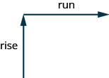
The slope of a line is \(m=\frac{\text{rise}}{\text{run}}\).
The rise measures the vertical change and the run measures the horizontal change.
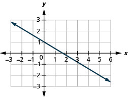
Find the slope of the line shown.
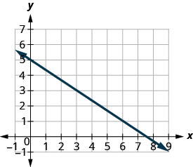
| Locate two points on the graph whose coordinates are integers. |
\((0,5)\) and \((3,3)\) |
| Starting at \((0,5)\), sketch a right triangle to \((3,3)\) as shown in this graph. |
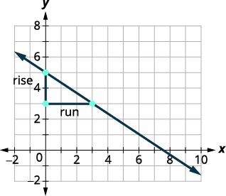 |
| Count the rise— since it goes down, it is negative. | The rise is \(−2\). |
| Count the run. We suggest always running to the right | The run is \(3\). |
| Use the slope formula. | \(m=\frac{\text{rise}}{\text{run}}\) |
| Substitute the values of the rise and run. | \(m=\frac{-2}{3}\) |
| Simplify. | \(m=−\frac{2}{3}\) |
| The slope of the line is \(−\frac{2}{3}\). | |
| So y decreases by 2 units as x increases by 3 units. |
| Notice what happens if we were to choose two different points whose coordinates are integers. | \((3,3)\) and \((6.1)\) |
| Count the rise and the run. | The rise is \(−2\). The run is \(3\) |
| Simplify. | \(m=−\frac{2}{3}\) |
| The slope of the line is \(−\frac{2}{3}\) regardless of which points you choose |
a. Find the slope of the line shown.
- Answer a
-
\(-\frac{4}{3}\)
b. Find the slope of the line shown.
- Answer b
-
\(-\frac{3}{5}\)
How do we find the slope of horizontal and vertical lines?
To find the slope of the horizontal line, \(y=4\), we could graph the line, find two points on it, and count the rise and the run. Let’s see what happens when we do this, as shown in the graph below.
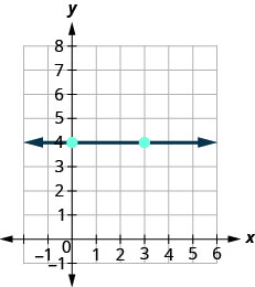
\( \begin{array}{ll} {\text{What is the rise?}} &{\text{The rise is 0 because it does not go up or down.}} \\ {\text{What is the run?}} &{\text{The run is }3.} \\ {\text{What is the slope?}} &{m=\frac{\text{rise}}{\text{run}}} \\ {} &{m=\frac{0}{3}} \\ {} &{m=0} \\{}&{\text{The slope of the horizontal line } y=4 \text{ is }0.} \\ \end{array} \nonumber\)
\( \begin{array}{cc} {\text{What is the rise?}} &{\text{The rise is 0 because it does not go up or down.}} \\ \end{array} \nonumber\)
Let’s also consider a vertical line, the line \(x=3\), as shown in the graph.
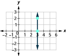
\( \begin{array}{ll} {\text{What is the rise?}} &{\text{The rise is }2.} \\ {\text{What is the run?}} &{\text{The run is 0 because it does not move right or left.}} \\ {\text{What is the slope?}} &{m=\frac{\text{rise}}{\text{run}}} \\ {} &{m=\frac{2}{0}} \\ \end{array} \nonumber\)
The slope is undefined since division by zero is undefined. So we say that the slope of the vertical line \(x=3\) is undefined.
All horizontal lines have slope \(0\). When the \(y\)-coordinates are the same, the rise is \(0\).
The slope of any vertical line is undefined. When the x-coordinates of a line are all the same, the run is \(0\) and we cannot divide by zero therefore the slope is undefined.
Find the slope of each line: a. \(x=8\) b. \(y=−5\).
Solution- \(x=8\) This is a vertical line. Its slope is undefined.
- \(y=−5\) This is a horizontal line. It has slope 0.
Sometimes we’ll need to find the slope of a line between two points without a graph to count out the rise and the run. We could plot the points on grid paper, then count out the rise and the run, but as we will see, there is a way to find the slope without graphing. Before we get to it, we need to introduce some algebraic notation.
We have seen that an ordered pair \((x,y)\) gives the coordinates of a point. But when we work with slopes, we use two points. How can the same symbol \((x,y)\) be used to represent two different points? Mathematicians use subscripts to distinguish the points.
\( \begin{array} {ll} {(x_1, y_1)} &{\text{read “} x \text{ sub } 1, \space y \text{ sub } 1 \text{”}} \\ {(x_2, y_2)} &{\text{read “} x \text{ sub } 2, \space y \text{ sub } 2 \text{”}} \\ \end{array} \nonumber\)
We will use \((x_1,y_1)\) to identify the first point and \((x_2,y_2)\) to identify the second point.
If we had more than two points, we could use \((x_3,y_3)\), \((x_4,y_4)\), and so on.
Let’s see how the rise and run relate to the coordinates of the two points by taking another look at the slope of the line between the points \((2,3)\) and \((7,6)\), as shown in this graph.
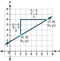
\( \begin{array} {ll} {\text{Since we have two points, we will use subscript notation.}} &{ \begin{pmatrix} x_1, & y_1 \\ 2 & 3 \end{pmatrix} \begin{pmatrix} x_2, & y_2 \\ 7 & 6 \end{pmatrix}} \\ {} &{m=\frac{\text{rise}}{\text{run}}} \\ {\text{On the graph, we counted the rise of 3 and the run of 5.}} &{m=\frac{3}{5}} \\ {\text{Notice that the rise of 3 can be found by subtracting the}} &{} \\ {y\text{-coordinates, 6 and 3, and the run of 5 can be found by}} &{} \\ {\text{subtracting the x-coordinates 7 and 2.}} &{} \\ {\text{We rewrite the rise and run by putting in the coordinates.}} &{m=\frac{6-3}{7-2}} \\ {} &{} \\ {\text{But 6 is } y_2 \text{, the y-coordinate of the second point and 3 is }y_1 \text{, the y-coordinate}} &{} \\ {\text{of the first point. So we can rewrite the slope using subscript notation.}} &{m=\frac{y_2-y_1}{7-2}} \\ {\text{Also 7 is the x-coordinate of the second point and 2 is the x-coordinate}} &{} \\ {\text{of the first point. So again we rewrite the slope using subscript notation.}} &{m=\frac{y_2-y_1}{x_2-x_1}} \\ \end{array} \nonumber\)
We have shown that \(m=\frac{y_2−y_1}{x_2−x_1}\) is really another version of \(m=\frac{\text{rise}}{\text{run}}\). We can use this formula to find the slope of a line when we have two points on the line.
a. Use the slope formula to find the slope of the line through the points \((−2,−3)\) and \((-7,4)\).
- Answer a
-
We will call \((−2,−3)\) point #1 and \((-7,4)\) point #2. Then, using the slope formula, we get
\(m=\dfrac{4-(-3)}{-7-(-2)}\)
\(m=-\frac{7}{5}\)
Let’s verify this slope on the graph shown.
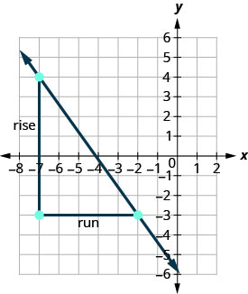
\[m=\frac{\text{rise}}{\text{run}} \nonumber\] \[m=\frac{7}{−5} \nonumber\] \[m=\frac{−7}{5} \nonumber\]
b. Use the slope formula to find the slope of the line through the pair of points: \((−3,4)\) and \((2,−1)\).
- Answer b
-
\(-1\)
Linear Equations
Up to now, all the equations you have solved were equations with just one variable. In almost every case, when you solved the equation you got exactly one solution. But equations can have more than one variable. Equations with two variables may be of the form \(Ax+By=C\). An equation of this form is called a linear equation in two variables.
Here is an example of a linear equation in two variables, \(x\) and \(y\).
\(\begin{align*} {\color{BrickRed}A}x + {\color{RoyalBlue}B}y &= {\color{forestgreen}C} \\[5pt]
x+{\color{RoyalBlue}4}y &= {\color{forestgreen}8} \end{align*}\)
\({\color{BrickRed}A = 1}\), \({\color{RoyalBlue}B = 4}\), \({\color{forestgreen}C=8}\)
The equation \(y=−3x+5\) is also a linear equation. But it does not appear to be in the form \(Ax+By=C\). We can use the Addition Property of Equality and rewrite it in \(Ax+By=C\) form.
\[ \begin{array} {lrll} {} &{y} &= &{-3x+5} \\ {\text{Add to both sides.} } &{y+3x} &= &{3x+5+3x} \\ {\text{Simplify.} } &{y+3x} &= &{5} \\ {\text{Use the Commutative Property to put it in} } &{} &{} &{} \\ {Ax+By=C\text{ form.} } &{3x+y} &= &{5} \end{array} \nonumber\]
By rewriting \(y=−3x+5\) as \(3x+y=5\), we can easily see that it is a linear equation in two variables because it is of the form \(Ax+By=C\). When an equation is in the form \(Ax+By=C\), we say it is in standard form of a linear equation.
Most people prefer to have \(A,\) \(B,\) and \(C\) be integers and \(A \geq 0\) when writing a linear equation in standard form, although it is not strictly necessary.
Linear equations have infinitely many solutions. For every number that is substituted for \(x\) there is a corresponding \(y\)-value. This pair of values is a solution to the linear equation and is represented by the ordered pair \((x,y)\). When we substitute these values of \(x\) and \(y\) into the equation, the result is a true statement, because the value on the left side is equal to the value on the right side.
Linear equations have infinitely many solutions. We can plot these solutions in the rectangular coordinate system. The points will line up perfectly in a straight line. We connect the points with a straight line to get the graph of the equation. We put arrows on the ends of each side of the line to indicate that the line continues in both directions.
Solutions to Linear Equations
A graph is a visual representation of all the solutions of the equation. It is an example of the saying, “A picture is worth a thousand words.” The line shows you all the solutions to that equation. Every point on the line is a solution of the equation. And, every solution of this equation is on this line. This line is called the graph of the equation. Points not on the line are not solutions!
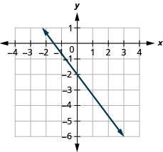
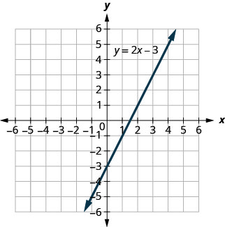
The graph of \(y=2x−3\) is shown.
For each ordered pair, decide:
- Is the ordered pair a solution to the equation?
- Is the point on the line?
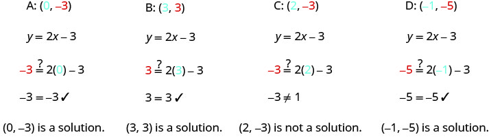
A: \((0,−3)\) B: \((3,3)\) C: \((2,−3)\) D: \((−1,−5)\)
Solution:
Substitute the \(x\)- and \(y\)-values into the equation to check if the ordered pair is a solution to the equation.
a.
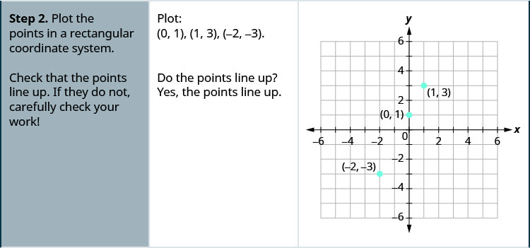
b. Plot the points \((0,−3)\), \((3,3)\), \((2,−3)\), and \((−1,−5)\).
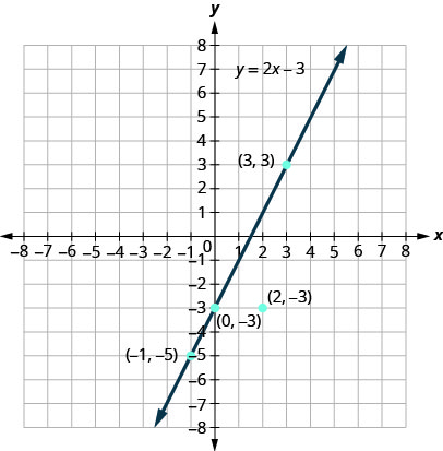
The points \((0,3)\), \((3,−3)\), and \((−1,−5)\) are on the line \(y=2x−3\), and the point \((2,−3)\) is not on the line.
The points that are solutions to \(y=2x−3\) are on the line, but the point that is not a solution is not on the line.
Graph a Linear Equation by Plotting Points
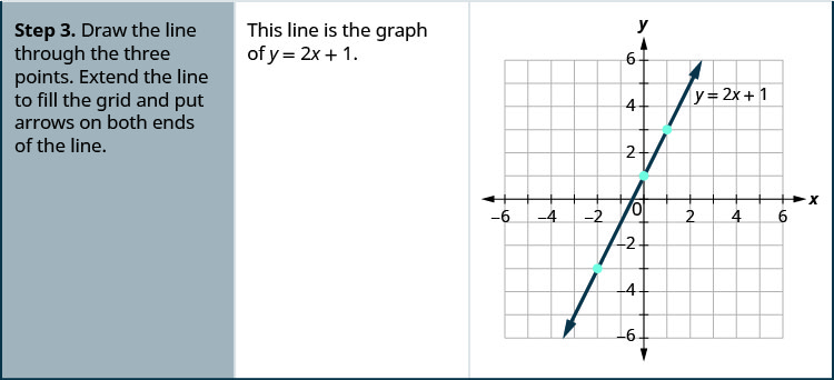
There are several methods that can be used to graph a linear equation. The first method we will use is called plotting points, or the Point-Plotting Method. We find three points whose coordinates are solutions to the equation and then plot them in a rectangular coordinate system. By connecting these points in a line, we have the graph of the linear equation.
Graph the equation \(y=2x+1\) by plotting points.
Solution:
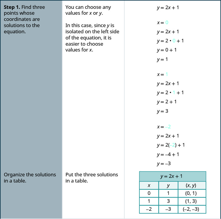
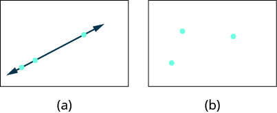
It is true that it only takes two points to determine a line, but it is a good habit to use three points. If you only plot two points and one of them is incorrect, you can still draw a line but it will not represent the solutions to the equation. It will be the wrong line.
If you use three points, and one is incorrect, the points will not line up. This tells you something is wrong and you need to check your work. Look at the difference between these illustrations.
When an equation includes a fraction as the coefficient of \(x,\) we can still substitute any numbers for \(x.\) But the arithmetic is easier if we make “good” choices for the values of \(x.\) This way we will avoid fractional answers, which are hard to graph precisely.
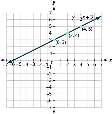
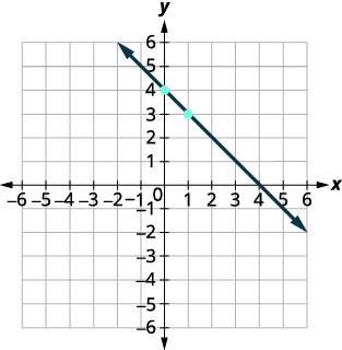
Graph the equation: \(y=\frac{1}{2}x+3\).
Solution:
Find three points that are solutions to the equation. Since this equation has the fraction \(\dfrac{1}{2}\) as a coefficient of \(x,\) we will choose values of \(x\) carefully. We will use zero as one choice and multiples of \(2\) for the other choices. Why are multiples of two a good choice for values of \(x\)? By choosing multiples of \(2\) the multiplication by \(\dfrac{1}{2}\) simplifies to a whole number
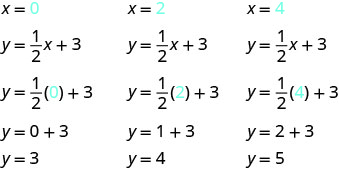
| \(y=\frac{1}{2}x+3\) | ||
| \(x\) | \(y\) | \((x,y)\) |
| 0 | 3 | \((0,3)\) |
| 2 | 4 | \((2,4)\) |
| 4 | 5 | \((4,5)\) |
Plot the points, check that they line up, and draw the line.
Graph a Line Given a Point and the Slope
Up to now, in this chapter, we have graphed lines by plotting points, by using intercepts, and by recognizing horizontal and vertical lines.
We can also graph a line when we know one point and the slope of the line. We will start by plotting the point and then use the definition of slope to draw the graph of the line.
Graph the line passing through the point \((1,−1)\) whose slope is \(m=\frac{3}{4}\).
Solution| Step 1. Plot the given point. | Plot \( (1, -1) \) |  |
| Step 2. Use the slope formula \( m=\dfrac{\text{rise}}{\text{run}} \) to identify the rise and the run. | Identify the rise and the run. | \( m = \dfrac{3}{4} \\ \) \( \dfrac{\text{rise}}{\text{run}} = \dfrac{3}{4} \\ \) rise = 3 run = 4 |
| Step 3. Starting at the given point, count out the rise and run to mark the second point. | Start at \( (1, -1) \) and count the rise and the run. Up \(3\) units, right \(4\) units. |  |
| Step 4. Connect the points with a line. | Connect the two points with a line. |  |
You can check your work by finding a third point. Since the slope is \(m=\frac{3}{4}\), it can also be written as \(m=\frac{−3}{−4}\) (negative divided by negative is positive!). Go back to \((1,−1)\) and count out the rise, \(−3\), and the run, \(−4\).
a. Graph the line passing through the point \((2,−2)\) with the slope \(m=\frac{4}{3}\).
- Answer a
-

b. Graph the line passing through the point \((1,1)\) with the slope \(m=-\frac{3}{5}\).
- Answer b
-

Graph Find \(x\)- and \(y\)-intercepts
Every linear equation can be represented by a unique line that shows all the solutions of the equation. We have seen that when graphing a line by plotting points, you can use any three solutions to graph. This means that two people graphing the line might use different sets of three points.
At first glance, their two lines might not appear to be the same, since they would have different points labeled. But if all the work was done correctly, the lines should be exactly the same. One way to recognize that they are indeed the same line is to look at where the line crosses the \(x\)-axis and the \(y\)-axis. These points are called the intercepts of a line.
Let’s look at the graphs of the lines.
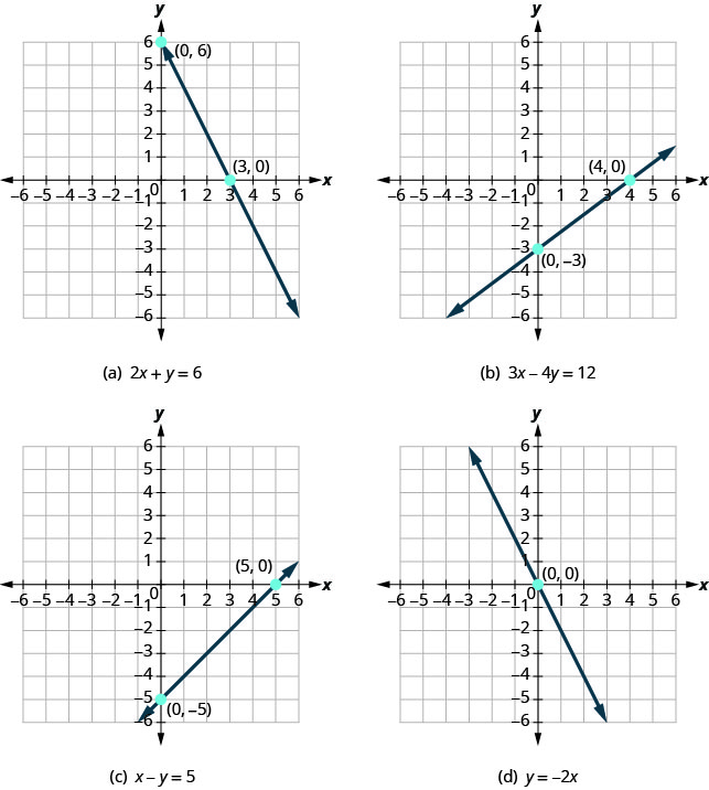
First, notice where each of these lines crosses the \(x\)-axis.
Now, let’s look at the points where these lines cross the \(y\)-axis.
| Figure | The line crosses the \(x\)-axis at: |
Ordered pair for this point |
The line crosses the y-axis at: |
Ordered pair for this point |
|---|---|---|---|---|
| Figure (a) | \(3\) | \((3,0)\) | \(6\) | \((0,6)\) |
| Figure (b) | \(4\) | \((4,0)\) | \(−3\) | \((0,−3)\) |
| Figure (c) | \(5\) | \((5,0)\) | \(−5\) | \((0,5)\) |
| Figure (d) | \(0\) | \((0,0)\) | \(0\) | \((0,0)\) |
| General Figure | \(a\) | \((a,0)\) | \(b\) | \((0,b)\) |
Do you see a pattern?
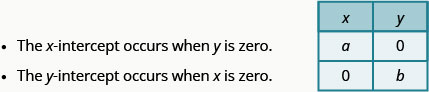
For each line, the \(y\)-coordinate of the point where the line crosses the \(x\)-axis is zero. The point where the line crosses the \(x\)-axis has the form \((a,0)\) and is called the \(x\)-intercept of the line. The \(x\)-intercept occurs when \(y\) is zero.
In each line, the \(x\)-coordinate of the point where the line crosses the \(y\)-axis is zero. The point where the line crosses the \(y\)-axis has the form \((0,b)\) and is called the \(y\)-intercept of the line. The \(y\)-intercept occurs when \(x\) is zero.
The \(x\)-intercept is the point \((a,0)\) where the line crosses the \(x\)-axis.
The \(y\)-intercept is the point \((0,b)\) where the line crosses the \(y\)-axis.
Recognizing that the \(x\)-intercept occurs when \(y\) is zero and that the \(y\)-intercept occurs when \(x\) is zero, gives us a method to find the intercepts of a line from its equation. To find the \(x\)-intercept, let \(y=0\) and solve for \(x.\) To find the \(y\)-intercept, let \(x=0\) and solve for \(y.\)
Find the intercepts of \(2x+y=8\).
- Answer
-
\(x\)-intercept: \((8,0)\),
Find the intercepts of \(2x+y=8\).
Solution:
We will let \(y=0\) to find the \(x\)-intercept, and let \(x=0\) to find the \(y\)-intercept. We will fill in a table, which reminds us of what we need to find.
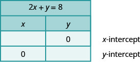
To find the \(x\)-intercept, let \(y=0\). \(2x+y=8\) Let \(y=0\). \(2x+{\color{red}0}=8\) Simplify. \(2x=8\) \(x=4\) The \(x\)-intercept is: \((4,0)\) To find the \(y\)-intercept, let \(x=0\). \(2x+y=8\) Let \(x=0\). \(2 ( {\color{red}0}) + y = 8\) Simplify. \(0 + y = 8\) \(y=8\) The \(y\)-intercept is: \((0,8)\) The intercepts are the points \((4,0)\) and \((0,8)\) as shown in the table.
\(2x+y=8\) \(x\) \(y\) 4 0 0 8
Find the \(x\)- and \(y\)-intercepts on each graph shown. 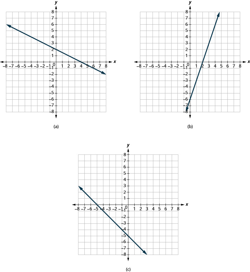
- Answer
-
a. The graph crosses the \(x\)-axis at the point \((4,0)\). The x-intercept is \((4,0)\).
The graph crosses the \(y\)-axis at the point \((0,2)\). The \(y\)-intercept is \((0,2)\).
b. The graph crosses the \(x\)-axis at the point \((2,0)\). The \(x\)-intercept is \((2,0)\).
The graph crosses the \(y\)-axis at the point \((0,−6)\). The \(y\)-intercept is \((0,−6)\).
c. The graph crosses the \(x\)-axis at the point \((−5,0)\). The \(x\)-intercept is \((−5,0)\).
The graph crosses the \(y\)-axis at the point \((0,−5)\). The \(y\)-intercept is \((0,−5)\).
Find the intercepts: \(x+4y=8\).
- Answer
-
\(x\)-intercept: \((8,0)\),
\(y\)-intercept: \((0,2)\)
Find the intercepts: \(x+4y=8\).
- Answer
-
\(x\)-intercept: \((8,0)\),
\(y\)-intercept: \((0,2)\)
Graph a Line Using Slope and Intercept
We have graphed linear equations by plotting points, using intercepts, recognizing horizontal and vertical lines, and using one point and the slope of the line. Once we see how an equation in slope–intercept form and its graph are related, we will have one more method we can use to graph lines.
Let’s look at the graph of the equation \(y=\frac{1}{2}+3\) and find its slope and y-intercept.
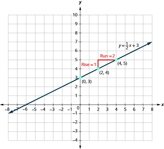
The red lines in the graph show us the rise is 1 and the run is 2. Substituting into the slope formula:
\[m=\frac{\text{rise}}{\text{run}} \nonumber\] \[m=\frac{1}{2} \nonumber\]
The y-intercept is \((0,3)\).
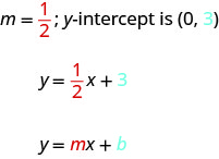
Look at the equation of this line. \(y = {\color{red}{\dfrac{1}{2}}}x+{\color{Cerulean}{3}} \)
Look at the slope and y-intercept. slope \( m = {\color{red}{\dfrac{1}{2}}} \) and y-intercept \( (0, {\color{Cerulean}{3}} ) \)
When a linear equation is solved for y, the coefficient of the x term is the slope and the constant term is the y-coordinate of the y-intercept. We say that the equation \(y=\frac{1}{2}x+3\) is in slope–intercept form. Sometimes the slope–intercept form is called the “y-form.”
The slope–intercept form of an equation of a line with slope m and y-intercept, \((0,b)\) is \(y=mx+b\).
Let’s practice finding the values of the slope and y-intercept from the equation of a line.
Identify the slope and y-intercept of the line from the equation: a. \(y=−\frac{4}{7}x−2\) b. \(x+3y=9\)
Solutiona. We compare our equation to the slope–intercept form of the equation.
| Write the slope–intercept form of the equation of the line. | \( y = {\color{red}{m}}x + \color{Cerulean}{b} \) |
| Write the equation of the line. | \( y = {\color{red}{-\dfrac{4}{7}}}x \color{Cerulean}{-2} \) |
| Identify the slope. | \( m = {\color{red}{-\dfrac{4}{7}}} \) |
| Identify the y-intercept. | y=intercept is \( (0, {\color{Cerulean}{-2}} ) \) |
b. When an equation of a line is not given in slope–intercept form, our first step will be to solve the equation for y.
| Solve for y. | \(x+3y=9\) |
| Subtract x from each side. | \( 3y = -x + 9 \) |
| Divide both sides by 3. | \( \dfrac{3y}{3} = \dfrac{-x + 9}{3} \) |
| Simplify. | \(y = -\dfrac{1}{3}x+3 \) |
| Write the slope–intercept form of the equation of the line. | \( y = {\color{red}{m}}x + \color{Cerulean}{b} \) |
| Write the equation of the line. | \( y = {\color{red}{-\dfrac{1}{3}}}x + \color{Cerulean}{3} \) |
| Identify the slope. | \( m = {\color{red}{-\dfrac{1}{3}}} \) |
| Identify the y-intercept. | y=intercept is \( (0, {\color{Cerulean}{3}} ) \) |
a. Identify the slope and y-intercept from the equation of the line. a. \(y=\frac{2}{5}x−1\) b. \(x+4y=8\)
- Answer a
-
- \(m=\frac{2}{5}\); \((0,−1)\)
- \(m=−\frac{1}{4}\); \((0,2)\)
b. Identify the slope and y-intercept from the equation of the line. a. \(y=−\frac{4}{3} x+1\) b. \(3x+2y=12\)
- Answer b
-
- \(m=−\frac{4}{3}\); \((0,1)\)
- \(m=−\frac{3}{2}\); \((0,6)\)
c. Graph the line of the equation \(y=−x+4\) using its slope and y-intercept.
- Answer c
-
\(y=mx+b\) The equation is in slope–intercept form. \(y=−x+4\) Identify the slope and y-intercept. \(m=−1\)
y-intercept is \((0,4)\)Plot the y-intercept. See the graph. Identify the rise over the run. \(m=\frac{−1}{1}\) Count out the rise and run to mark the second point. rise \(-1\), run \(1\)
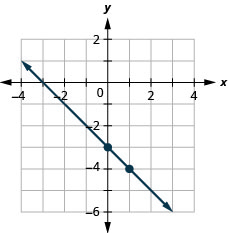
d . Graph the line of the equation \(y=−x−3\) using its slope and y-intercept.
- Answer d
-
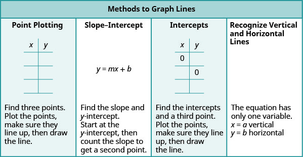
Now that we have graphed lines by using the slope and y-intercept, let’s summarize all the methods we have used to graph lines.

Choose the Most Convenient Method to Graph a Line
Now that we have seen several methods we can use to graph lines, how do we know which method to use for a given equation?
While we could plot points, use the slope–intercept form, or find the intercepts for any equation, if we recognize the most convenient way to graph a certain type of equation, our work will be easier.
Generally, plotting points is not the most efficient way to graph a line. Let’s look for some patterns to help determine the most convenient method to graph a line.
Here are five equations we graphed in this chapter, and the method we used to graph each of them.
\[ \begin{array} {lll} {} &{\textbf{Equation}} &{\textbf{Method}} \\ {\text{1)}} &{x=2} &{\text{Vertical line}} \\ {\text{2)}} &{y=−1} &{\text{Horizontal line}} \\ {\text{3)}} &{−x+2y=6} &{\text{Intercepts}} \\ {\text{4)}} &{4x−3y=12} &{\text{Intercepts}} \\ {\text{5)}} &{y=−x+4} &{\text{Slope–intercept}} \\ \end{array} \nonumber\]
Equations #1 and #2 each have just one variable. Remember, in equations of this form the value of that one variable is constant; it does not depend on the value of the other variable. Equations of this form have graphs that are vertical or horizontal lines.
In equations #3 and #4, both x and y are on the same side of the equation. These two equations are of the form \(Ax+By=C\). We substituted \(y=0\) to find the x- intercept and \(x=0\) to find the y-intercept and connected the twop points.
Equation #5 is written in slope–intercept form. After identifying the slope and y-intercept from the equation we used them to graph the line.
This leads to the following strategy.
Consider the form of the equation.
- If it only has one variable, it is a vertical or horizontal line.
- \(x=a\) is a vertical line passing through the x-axis at a.
- \(y=b\) is a horizontal line passing through the y-axis at b.
- If y is isolated on one side of the equation, in the form \(y=mx+b\), graph by using the slope and y-intercept.
- Identify the slope and y-intercept and then graph.
- If the equation is of the form \(Ax+By=C\), find the intercepts.
- Find the x- and y-intercepts, and then graph.
Determine the most convenient method to graph each line:
a. \(y=5\)
b. \(4x−5y=20\)
c. \(x=−3\)
d. \(y=−\frac{5}{9}x+8\)
e. \(x=6\)
f. \(y=−\frac{3}{4}x+1\)
g. \(4x−3y=−1\)
- Answer
-
a. \(y=5\) This equation has only one variable, y. Its graph is a horizontal line crossing the y-axis at \(5\).
b. \(4x−5y=20\) This equation is of the form \(Ax+By=C\). The easiest way to graph it will be to find the intercepts and one more point.
c. \(x=−3\) There is only one variable, x. The graph is a vertical line crossing the x-axis at \(−3\).
d. \(y=−\frac{5}{9}x+8\) Since this equation is in \(y=mx+b\) form, it will be easiest to graph this line by using the slope and y-intercepts.
e. vertical line
f. slope-intercept
g. intercepts
Use Slopes to Identify Parallel and Perpendicular Lines
Two lines that have the same slope are called parallel lines. Parallel lines have the same steepness and never intersect.
We say this more formally in terms of the rectangular coordinate system. Two lines that have the same slope and different y-intercepts are called parallel lines.
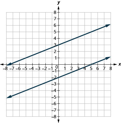
Verify that both lines have the same slope, \(m=\frac{2}{5}\), and different y-intercepts.
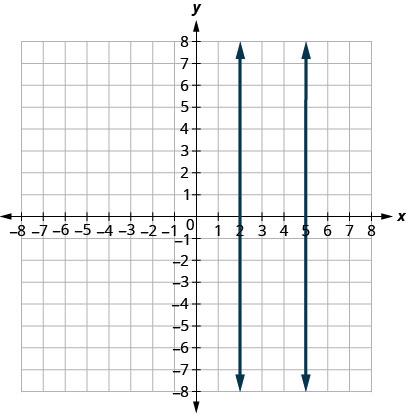
What about vertical lines? The slope of a vertical line is undefined, so vertical lines don’t fit in the definition above. We say that vertical lines that have different x-intercepts are parallel, like the lines shown in this graph.
Since parallel lines have the same slope and different y-intercepts, we can now just look at the slope–intercept form of the equations of lines and decide if the lines are parallel.
Use slopes and y-intercepts to determine if the lines are parallel:
a. \(3x−2y=6\) and \(y=\frac{3}{2}x+1\)
b. \(y=2x−3\) and \(−6x+3y=−9\).
- Answer
-
a.
\( \begin{array} {llll} {} &{3x−2y=6} &{\text{and}} &{y=\frac{3}{2}x+1} \\ {} &{−2y=−3x+6} &{} &{} \\ {\text{Solve the first equation for y.}} &{\frac{-2y}{-2}=\frac{-3x+6}{-2}} &{} &{} \\ {\text{The equation is now in slope–intercept form.}} &{y=\frac{3}{2}x−3} &{} &{} \\ {\text{The equation of the second line is already}} &{} &{} &{} \\ {\text{in slope–intercept form.}} &{} &{} &{y=\frac{3}{2}x+1} \\ {} &{} &{} &{} \\ {} &{y=\frac{3}{2}x−3} &{} &{y=\frac{3}{2}x+1} \\ {Identify the slope andy-intercept of both lines.} &{y=mx+b} &{} &{y=mx+b} \\ {} &{m=\frac{3}{2}} &{} &{y=\frac{3}{2}} \\ {} &{\text{y-intercept is }(0,−3)} &{} &{\text{y-intercept is }(0,1)} \\ \end{array} \nonumber\)
The lines have the same slope and different y-intercepts and so they are parallel.
You may want to graph the lines to confirm whether they are parallel.
b.
\( \begin{array} {llll} {} &{y=2x−3} &{\text{and}} &{−6x+3y=−9} \\ {\text{The first equation is already in slope–intercept form.}} &{y=2x−3} &{} &{} \\ {} &{} &{} &{−6x+3y=−9} \\ {} &{} &{} &{3y=6x−9} \\ {\text{Solve the second equation for y.}} &{} &{} &{\frac{3y}{3}=\frac{6x−9}{3}} \\ {} &{} &{} &{y=2x−3} \\ {\text{The second equation is now in slope–intercept form.}} &{} &{} &{y=2x−3} \\ {} &{} &{} &{} \\ {} &{y=2x−3} &{} &{y=2x−3} \\ {\text{Identify the slope andy-intercept of both lines.}} &{y=mx+b} &{} &{y=mx+b} \\ {} &{m=2} &{} &{m=2} \\ {} &{\text{y-intercept is }(0,−3)} &{} &{\text{y-intercept is }(0,-3)} \\ \end{array} \nonumber\)
The lines have the same slope, but they also have the same y-intercepts. Their equations represent the same line and we say the lines are coincident.
c. \(2x+5y=5\) and \(y=−\frac{2}{5}x−4\)
d. \(y=−\frac{1}{2}x−1\) and \(x+2y=−2\).
- Answer
-
c. parallel
d. not parallel; same line as they have the exact same intercepts and slope.
Let’s look at the lines whose equations are \(y=\frac{1}{4}x−1\) and \(y=−4x+2\).

These lines lie in the same plane and intersect in right angles. We call these lines perpendicular.
If we look at the slope of the first line, \(m_1=\frac{1}{4}\), and the slope of the second line, \(m_2=−4\), we can see that they are negative reciprocals of each other. If we multiply them, their product is \(−1\).
\[\begin{array} {l} {m_1·m_2} \\ {14(−4)} \\ {−1} \\ \end{array} \nonumber\]
This is always true for perpendicular lines and leads us to this definition.
We were able to look at the slope–intercept form of linear equations and determine whether or not the lines were parallel. We can do the same thing for perpendicular lines.
We find the slope–intercept form of the equation, and then see if the slopes are opposite reciprocals. If the product of the slopes is \(−1\), the lines are perpendicular.
Use slopes to determine if the lines are perpendicular:
a. \(y=−5x−4\) and \(x−5y=5\)
b. \(7x+2y=3\) and \(2x+7y=5\)
- Answer
-
a.
The first equation is in slope–intercept form.Solve the second equation fory.Identify the slope of each line.y=−5x−4yym1=−5x−4=mx+b=−5x−5y−5y−5y−5y=5=−x+5=−x+5−5=15x−1yym2=15x−1=mx+b=15The first equation is in slope–intercept form.y=−5x−4Solve the second equation fory.x−5y=5−5y=−x+5−5y−5=−x+5−5y=15x−1Identify the slope of each line.y=−5x−4y=mx+bm1=−5y=15x−1y=mx+bm2=15
The slopes are negative reciprocals of each other, so the lines are perpendicular. We check by multiplying the slopes, Since −5(15)=−1,−5(15)=−1, it checks.
b.
Solve the equations fory.Identify the slope of each line.7x+2y2y2y2y=3=−7x+3=−7x+32=−72x+32ym1=mx+b=−722x+7y7y7y7y=5=−2x+5=−2x+57=−27x+57ym1=mx+b=−27Solve the equations fory.7x+2y=32y=−7x+32y2=−7x+32y=−72x+322x+7y=57y=−2x+57y7=−2x+57y=−27x+57Identify the slope of each line.y=mx+bm1=−72y=mx+bm1=−27
The slopes are reciprocals of each other, but they have the same sign. Since they are not negative reciprocals, the lines are not perpendicular.
c. \(y=−3x+2\) and \(x−3y=4\)
d. \(5x+4y=1\) and \(4x+5y=3\).
- Answer
-
c. perpendicular
d. not perpendicular
Key Concepts
- Slope of a Line
- The slope of a line is \(m=\frac{\text{rise}}{\text{run}}\).
- The rise measures the vertical change and the run measures the horizontal change.
- How to find the slope of a line from its graph using \(m=\frac{\text{rise}}{\text{run}}\).
- Locate two points on the line whose coordinates are integers.
- Starting with one point, sketch a right triangle, going from the first point to the second point.
- Count the rise and the run on the legs of the triangle.
- Take the ratio of rise to run to find the slope: \(m=\frac{\text{rise}}{\text{run}}\).
- Slope of a line between two points.
- The slope of the line between two points \((x_1,y_1)\) and \((x_2,y_2)\) is:
\[m=\frac{y_2−y_1}{x_2−x_1} \nonumber\].
- The slope of the line between two points \((x_1,y_1)\) and \((x_2,y_2)\) is:
- How to graph a line given a point and the slope.
- Plot the given point.
- Use the slope formula \(m=\frac{\text{rise}}{\text{run}}\) to identify the rise and the run.
- Starting at the given point, count out the rise and run to mark the second point.
- Connect the points with a line.
- Slope Intercept Form of an Equation of a Line
- The slope–intercept form of an equation of a line with slope m and y-intercept, \((0,b)\) is \(y=mx+b\)
- Parallel Lines
- Parallel lines are lines in the same plane that do not intersect.
Parallel lines have the same slope and different y-intercepts.
If \(m_1\) and \(m_2\) are the slopes of two parallel lines then \(m_1=m_2\).
Parallel vertical lines have different x-intercepts.
- Parallel lines are lines in the same plane that do not intersect.
- Perpendicular Lines
- Perpendicular lines are lines in the same plane that form a right angle.
- If \(m_1\) and \(m_2\) are the slopes of two perpendicular lines, then:
their slopes are negative reciprocals of each other, \(m_1=−\frac{1}{m_2}\).
the product of their slopes is \(−1\), \(m_1·m_2=−1\). - A vertical line and a horizontal line are always perpendicular to each other.