
1.8: Slope-Intercept, Point-Slope, Standard form of lines, Vertical, Horizontal, Parallel, Perpendicular Lines and Applications
- Page ID
- 193549

\( \newcommand{\vecs}[1]{\overset { \scriptstyle \rightharpoonup} {\mathbf{#1}} } \)
\( \newcommand{\vecd}[1]{\overset{-\!-\!\rightharpoonup}{\vphantom{a}\smash {#1}}} \)
\( \newcommand{\dsum}{\displaystyle\sum\limits} \)
\( \newcommand{\dint}{\displaystyle\int\limits} \)
\( \newcommand{\dlim}{\displaystyle\lim\limits} \)
\( \newcommand{\id}{\mathrm{id}}\) \( \newcommand{\Span}{\mathrm{span}}\)
( \newcommand{\kernel}{\mathrm{null}\,}\) \( \newcommand{\range}{\mathrm{range}\,}\)
\( \newcommand{\RealPart}{\mathrm{Re}}\) \( \newcommand{\ImaginaryPart}{\mathrm{Im}}\)
\( \newcommand{\Argument}{\mathrm{Arg}}\) \( \newcommand{\norm}[1]{\| #1 \|}\)
\( \newcommand{\inner}[2]{\langle #1, #2 \rangle}\)
\( \newcommand{\Span}{\mathrm{span}}\)
\( \newcommand{\id}{\mathrm{id}}\)
\( \newcommand{\Span}{\mathrm{span}}\)
\( \newcommand{\kernel}{\mathrm{null}\,}\)
\( \newcommand{\range}{\mathrm{range}\,}\)
\( \newcommand{\RealPart}{\mathrm{Re}}\)
\( \newcommand{\ImaginaryPart}{\mathrm{Im}}\)
\( \newcommand{\Argument}{\mathrm{Arg}}\)
\( \newcommand{\norm}[1]{\| #1 \|}\)
\( \newcommand{\inner}[2]{\langle #1, #2 \rangle}\)
\( \newcommand{\Span}{\mathrm{span}}\) \( \newcommand{\AA}{\unicode[.8,0]{x212B}}\)
\( \newcommand{\vectorA}[1]{\vec{#1}} % arrow\)
\( \newcommand{\vectorAt}[1]{\vec{\text{#1}}} % arrow\)
\( \newcommand{\vectorB}[1]{\overset { \scriptstyle \rightharpoonup} {\mathbf{#1}} } \)
\( \newcommand{\vectorC}[1]{\textbf{#1}} \)
\( \newcommand{\vectorD}[1]{\overrightarrow{#1}} \)
\( \newcommand{\vectorDt}[1]{\overrightarrow{\text{#1}}} \)
\( \newcommand{\vectE}[1]{\overset{-\!-\!\rightharpoonup}{\vphantom{a}\smash{\mathbf {#1}}}} \)
\( \newcommand{\vecs}[1]{\overset { \scriptstyle \rightharpoonup} {\mathbf{#1}} } \)
\(\newcommand{\longvect}{\overrightarrow}\)
\( \newcommand{\vecd}[1]{\overset{-\!-\!\rightharpoonup}{\vphantom{a}\smash {#1}}} \)
\(\newcommand{\avec}{\mathbf a}\) \(\newcommand{\bvec}{\mathbf b}\) \(\newcommand{\cvec}{\mathbf c}\) \(\newcommand{\dvec}{\mathbf d}\) \(\newcommand{\dtil}{\widetilde{\mathbf d}}\) \(\newcommand{\evec}{\mathbf e}\) \(\newcommand{\fvec}{\mathbf f}\) \(\newcommand{\nvec}{\mathbf n}\) \(\newcommand{\pvec}{\mathbf p}\) \(\newcommand{\qvec}{\mathbf q}\) \(\newcommand{\svec}{\mathbf s}\) \(\newcommand{\tvec}{\mathbf t}\) \(\newcommand{\uvec}{\mathbf u}\) \(\newcommand{\vvec}{\mathbf v}\) \(\newcommand{\wvec}{\mathbf w}\) \(\newcommand{\xvec}{\mathbf x}\) \(\newcommand{\yvec}{\mathbf y}\) \(\newcommand{\zvec}{\mathbf z}\) \(\newcommand{\rvec}{\mathbf r}\) \(\newcommand{\mvec}{\mathbf m}\) \(\newcommand{\zerovec}{\mathbf 0}\) \(\newcommand{\onevec}{\mathbf 1}\) \(\newcommand{\real}{\mathbb R}\) \(\newcommand{\twovec}[2]{\left[\begin{array}{r}#1 \\ #2 \end{array}\right]}\) \(\newcommand{\ctwovec}[2]{\left[\begin{array}{c}#1 \\ #2 \end{array}\right]}\) \(\newcommand{\threevec}[3]{\left[\begin{array}{r}#1 \\ #2 \\ #3 \end{array}\right]}\) \(\newcommand{\cthreevec}[3]{\left[\begin{array}{c}#1 \\ #2 \\ #3 \end{array}\right]}\) \(\newcommand{\fourvec}[4]{\left[\begin{array}{r}#1 \\ #2 \\ #3 \\ #4 \end{array}\right]}\) \(\newcommand{\cfourvec}[4]{\left[\begin{array}{c}#1 \\ #2 \\ #3 \\ #4 \end{array}\right]}\) \(\newcommand{\fivevec}[5]{\left[\begin{array}{r}#1 \\ #2 \\ #3 \\ #4 \\ #5 \\ \end{array}\right]}\) \(\newcommand{\cfivevec}[5]{\left[\begin{array}{c}#1 \\ #2 \\ #3 \\ #4 \\ #5 \\ \end{array}\right]}\) \(\newcommand{\mattwo}[4]{\left[\begin{array}{rr}#1 \amp #2 \\ #3 \amp #4 \\ \end{array}\right]}\) \(\newcommand{\laspan}[1]{\text{Span}\{#1\}}\) \(\newcommand{\bcal}{\cal B}\) \(\newcommand{\ccal}{\cal C}\) \(\newcommand{\scal}{\cal S}\) \(\newcommand{\wcal}{\cal W}\) \(\newcommand{\ecal}{\cal E}\) \(\newcommand{\coords}[2]{\left\{#1\right\}_{#2}}\) \(\newcommand{\gray}[1]{\color{gray}{#1}}\) \(\newcommand{\lgray}[1]{\color{lightgray}{#1}}\) \(\newcommand{\rank}{\operatorname{rank}}\) \(\newcommand{\row}{\text{Row}}\) \(\newcommand{\col}{\text{Col}}\) \(\renewcommand{\row}{\text{Row}}\) \(\newcommand{\nul}{\text{Nul}}\) \(\newcommand{\var}{\text{Var}}\) \(\newcommand{\corr}{\text{corr}}\) \(\newcommand{\len}[1]{\left|#1\right|}\) \(\newcommand{\bbar}{\overline{\bvec}}\) \(\newcommand{\bhat}{\widehat{\bvec}}\) \(\newcommand{\bperp}{\bvec^\perp}\) \(\newcommand{\xhat}{\widehat{\xvec}}\) \(\newcommand{\vhat}{\widehat{\vvec}}\) \(\newcommand{\uhat}{\widehat{\uvec}}\) \(\newcommand{\what}{\widehat{\wvec}}\) \(\newcommand{\Sighat}{\widehat{\Sigma}}\) \(\newcommand{\lt}{<}\) \(\newcommand{\gt}{>}\) \(\newcommand{\amp}{&}\) \(\definecolor{fillinmathshade}{gray}{0.9}\)- Write linear equations
- Use linear equations to solve real-world problems.
- Apply slope to rates of change
- Write the equation of a line parallel or perpendicular to a given line
Linear equations are everywhere in the real world. When you try to figure how long it will take you to get home while driving a certain speed, or determining if you have enough money to pay your bills, you are solving a linear equation. In this section, we will practice solving some linear equations, create linear equations from given information, and examine applications of linear equations and slope intercept form. Usually, when a linear equation model uses real-world data, different letters are used for the variables, instead of using only x and y but you will still use the concept of slope and \(y\)-intercept (starting value or initial condition).
Finding a Linear Equation
Perhaps the most familiar form of a linear equation is the slope-intercept form, written as \[y=mx+b\] where \(m=\text{slope}\) and \(b=\text{y−intercept.}\) Let us begin with the slope.
The slope of a line refers to the ratio of the vertical change in \(y\) over the horizontal change in \(x\) between any two points on a line. It indicates the direction in which a line slants as well as its steepness. Slope is sometimes described as rise over run.
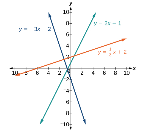
If the slope is positive, the line slants to the right. If the slope is negative, the line slants to the left. As the slope increases, the line becomes steeper. Some examples are shown in Figure \(\PageIndex{1}\). The lines indicate the following slopes: \(m=−3\), \(m=2\), and \(m=\dfrac{1}{3}\).
Let's take a minute and practice writing lines in slope-intercept form.
a. Given a slope of \(-\frac{2}{3}\) and a \(y\)-intercept of \(6\), write the equation of the line in slope-intercept form. Then graph the equation.
- Answer a
-
It will be in your best interest to memorize that slope-intercept form of a line is \(y=mx+b\) where \(m\) is the slope of the line and \(b\) is the \(y\)-intercept, the initial condition, or the point of the form \((0,y)\).
This line will have the equation \(y=-\frac{2}{3}x+6\). Notice on the graph below, the \(y\)-intercept is at \((0,6)\). Starting at the \(y\)-intercept, you can count down two and right three to find the next point on the line.

b. Given a slope of \(-\frac{2}{3}\) and the point \((3,6)\), write the equation of the line in slope-intercept form. Then graph the equation.
- Answer b
-
Starting with the equation \(y=mx+b\) we will substitute in with the given information. We know that \(y=6\) and \(x=3\) from the ordered pair and we know that \(m=-\frac{2}{3}\) since \(m\)=slope.
We now have the equation \(6=-\frac{2}{3}(3)+b\)
\(6=-2+b\)
\(8=b\)
The equation of the line is \(y=-\frac{2}{3}x+8\).
Notice this line has the same slope as in part a, but it has a different \(y\)-intercept. Since they have the same slope, these two lines are parallel.
c. Given the point \((-2,5)\) and the point \((2,1)\), write the equation of the line in slope-intercept form.
- Answer c
-
We find the slope between the two points by using \(m=\frac{y_2-y_1}{x_2-x_1}\) = \(m=\frac{1-5}{2-(-2)}\) \(=m=\frac{-4}{4}\)
Notice it does NOT matter which point you choose first as long as you are consistent. \(m=\frac{5-1}{-2-2}\) \(=m=\frac{4}{-4}\)
Now we may choose either point, I prefer not to deal with the negative signs so I will choose \((2,1)\) to go with \(m=-1\)
\(1=-(1)(2)+b\)
\(1=-2+b\)
\(-3=b\)
The equation of the line is \(y=1x-3\).
d. Given the point \((6,2)\) and the point \((8,5)\), write the equation of the line in slope-intercept form.
- Answer d
-
We find the slope between the two points by using \(m=\frac{y_2-y_1}{x_2-x_1}\) = \(m=\frac{5-2}{8-6}\) \(=m=\frac{3}{2}\)
Now we may choose either point, let's choose \((6,2)\) to go with \(m=\frac{3}{2}\)
\(2=\frac{3}{2}(6)+b\)
\(2=9+b\)
\(-7=b\)
The equation of the line is \(y=\frac{3}{2}x-7\)
What do you notice about the slope of this line compared to the line in a.
Graph and see what you notice about the relationship between the two lines.
There are two cell phone companies that offer different packages. Company A charges a monthly service fee of \($34\) plus \($.05/min\) talk-time. Company B charges a monthly service fee of \($40\) plus \($.04/min\) talk-time.
- Write a linear equation that models the packages offered by both companies.
- If the average number of minutes used each month is \(1,160\), which company offers the better plan?
- If the average number of minutes used each month is \(420\), which company offers the better plan?
- How many minutes of talk-time would yield equal monthly statements from both companies?
- Answer
-
a.
The model for Company A can be written as \( A =0.05x+34\). This includes the variable cost of \( 0.05x\) plus the monthly service charge of \($34\). Company B’s package charges a higher monthly fee of \($40\), but a lower variable cost of \( 0.04x\). Company B’s model can be written as \( B =0.04x+$40\).
b.
If the average number of minutes used each month is \(1,160\), we have the following:
\[\begin{align*} \text{Company A}&= 0.05(1.160)+34\\ &= 58+34\\ &= 92 \end{align*}\]
\[\begin{align*} \text{Company B}&= 0.04(1,1600)+40\\ &= 46.4+40\\ &= 86.4 \end{align*}\]
So, Company B offers the lower monthly cost of \($86.40\) as compared with the \($92\) monthly cost offered by Company A when the average number of minutes used each month is \(1,160\).
c.
If the average number of minutes used each month is \(420\), we have the following:
\[\begin{align*} \text{Company A}&= 0.05(420)+34\\ &= 21+34\\ &= 55 \end{align*}\]
\[\begin{align*} \text{Company B}&= 0.04(420)+40\\ &= 16.8+40\\ &= 56.8 \end{align*}\]
If the average number of minutes used each month is \(420\), then Company A offers a lower monthly cost of \($55\) compared to Company B’s monthly cost of \($56.80\).
d.
To answer the question of how many talk-time minutes would yield the same bill from both companies, we should think about the problem in terms of \((x,y)\) coordinates: At what point are both the \(x\)-value and the \(y\)-value equal? We can find this point by setting the equations equal to each other and solving for \(x\).
\[\begin{align*} 0.05x+34&= 0.04x+40\\ 0.01x&= 6\\ x&= 600 \end{align*}\]Check the \(x\)-value in each equation.
\(0.05(600)+34=64\)
\(0.04(600)+40=64\)
Therefore, a monthly average of \(600\) talk-time minutes renders the plans equal. See Figure \(\PageIndex{2}\).
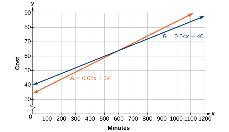
Figure \(\PageIndex{2}\)
Interpret Applications of Linear Equations
We will examine a few applications here so you can see how equations written in slope-intercept form relate to real-world situations.
Usually, when a linear equation model uses real-world data, different letters are used for the variables, instead of using only x and y. The variable names remind us of what quantities are being measured.
Additionally, we often need to extend the axes in our rectangular coordinate system to accommodate larger positive and negative numbers to represent the data in the application.
The equation \(F=\frac{9}{5}C+32\) is used to convert temperatures, C, on the Celsius scale to temperatures, F, on the Fahrenheit scale.
a. Find the Fahrenheit temperature for a Celsius temperature of \(0\).
b. Find the Fahrenheit temperature for a Celsius temperature of \(20\).
c. Interpret the slope and F-intercept of the equation.
d. Graph the equation.
- Answer
-
a. \( \begin{array} {ll} {\text{Find the Fahrenheit temperature for a Celsius temperature of 0.}} &{F=\frac{9}{5}C+32} \\ {\text{Find F when C=0.}} &{F=\frac{9}{5}(0)+32} \\ {\text{Simplify.}} &{F=32} \\ \end{array} \nonumber\)
b. \( \begin{array} {ll} {\text{Find the Fahrenheit temperature for a Celsius temperature of 20.}} &{F=\frac{9}{5}C+32} \\ {\text{Find F when C=20.}} &{F=\frac{9}{5}(20)+32} \\ {\text{Simplify.}} &{F=36+32} \\ {\text{Simplify.}} &{F=68} \\ \end{array} \nonumber\)
c. Interpret the slope and F-intercept of the equation.
Even though this equation uses F and C, it is still in slope-intercept form.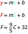
The slope, \(frac{9}{5}\), means that the temperature Fahrenheit (F) increases 9 degrees when the temperature Celsius (C) increases 5 degrees.
The F-intercept means that when the temperature is \(0°\) on the Celsius scale, it is \(32°\) on the Fahrenheit scale.
d. Graph the equation.
We’ll need to use a larger scale than our usual. Start at the F-intercept \((0,32)\), and then count out the rise of 9 and the run of 5 to get a second point as shown in the graph.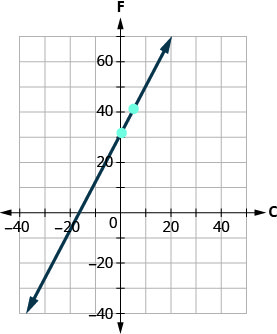
The equation \(h=2s+50\) is used to estimate a woman’s height in inches, h, based on her shoe size, s.
a. Estimate the height of a child who wears women’s shoe size \(0\).
b. Estimate the height of a woman with shoe size \(8\).
c. Interpret the slope and h-intercept of the equation.
d. Graph the equation.
- Answer
-
a. \(50\) inches
b. \(66\) inches
c. The slope, \(2\), means that the height, h, increases by \(2\) inches when the shoe size, s, increases by \(1\). The h-intercept means that when the shoe size is \(0\), the height is \(50\) inches.
d.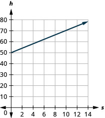
The equation \(T=\frac{1}{4}n+40\) is used to estimate the temperature in degrees Fahrenheit, T, based on the number of cricket chirps, n, in one minute.
a. Estimate the temperature when there are no chirps.
b. Estimate the temperature when the number of chirps in one minute is \(100\).
c. Interpret the slope and T-intercept of the equation.
d. Graph the equation.
- Answer
-
a. \(40\) degrees
b. \(65\) degrees
c. The slope, \(\frac{1}{4}\), means that the temperature Fahrenheit (F) increases \(1\) degree when the number of chirps, n, increases by \(4\). The T-intercept means that when the number of chirps is \(0\), the temperature is \(40°\).
d.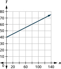
Setting up a Linear Equation to Solve a Real-World Application
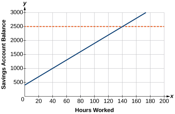
Caroline is a full-time college student planning a spring break vacation. To earn enough money for the trip, she has taken a part-time job at the local bank that pays \($15.00/hr\), and she opened a savings account with an initial deposit of \($400\) on January 15. She arranged for direct deposit of her payroll checks. If spring break begins March 20 and the trip will cost approximately \($2,500\), how many hours will she have to work to earn enough to pay for her vacation? If she can only work \(4\) hours per day, how many days per week will she have to work? How many weeks will it take? In this section, we will investigate problems like this and others, which generate graphs like the line in Figure \(\PageIndex{3}\).
Many real-world applications can be modeled by linear equations. For example, a cell phone package may include a monthly service fee plus a charge per minute of talk-time; it costs a widget manufacturer a certain amount to produce x widgets per month plus monthly operating charges; a car rental company charges a daily fee plus an amount per mile driven. These are examples of applications we come across every day that are modeled by linear equations. In this section, we will set up and use linear equations to solve such problems.
To set up or model a linear equation to fit a real-world application, we must first determine the independent and dependent variables. Then, we begin to interpret the words as mathematical expressions using mathematical symbols. Let us use the car rental example above. In this case, a known cost, such as \($0.10/mi\), is multiplied by an unknown quantity, the number of miles driven. Therefore, we can write \(0.10x\). This expression represents a variable cost because it changes according to the number of miles driven.
If a quantity is independent of a variable, we usually add or subtract it, according to the problem. As these amounts do not change, we refer to them as fixed costs. Consider a car rental agency that charges \($0.10/mi\) plus a daily fee of \($50\). We can use these quantities to model an equation that can be used to find the daily car rental cost \(C\).
\(C=0.10x+50 \tag{2.4.1}\)
There are two cell phone companies that offer different packages. Company A charges a monthly service fee of \($34\) plus \($.05/min\) talk-time. Company B charges a monthly service fee of \($40\) plus \($.04/min\) talk-time.
- Write a linear equation that models the packages offered by both companies.
- If the average number of minutes used each month is \(1,160\), which company offers the better plan?
- If the average number of minutes used each month is \(420\), which company offers the better plan?
- How many minutes of talk-time would yield equal monthly statements from both companies?
Solution
a.
The model for Company A can be written as \( A =0.05x+34\). This includes the variable cost of \( 0.05x\) plus the monthly service charge of \($34\). Company B’s package charges a higher monthly fee of \($40\), but a lower variable cost of \( 0.04x\). Company B’s model can be written as \( B =0.04x+$40\).
b.
If the average number of minutes used each month is \(1,160\), we have the following:
\[\begin{align*} \text{Company A}&= 0.05(1.160)+34\\ &= 58+34\\ &= 92 \end{align*}\]
\[\begin{align*} \text{Company B}&= 0.04(1,1600)+40\\ &= 46.4+40\\ &= 86.4 \end{align*}\]
So, Company B offers the lower monthly cost of \($86.40\) as compared with the \($92\) monthly cost offered by Company A when the average number of minutes used each month is \(1,160\).
c.
If the average number of minutes used each month is \(420\), we have the following:
\[\begin{align*} \text{Company A}&= 0.05(420)+34\\ &= 21+34\\ &= 55 \end{align*}\]
\[\begin{align*} \text{Company B}&= 0.04(420)+40\\ &= 16.8+40\\ &= 56.8 \end{align*}\]
If the average number of minutes used each month is \(420\), then Company A offers a lower monthly cost of \($55\) compared to Company B’s monthly cost of \($56.80\).
d.
To answer the question of how many talk-time minutes would yield the same bill from both companies, we should think about the problem in terms of \((x,y)\) coordinates: At what point are both the \(x\)-value and the \(y\)-value equal? We can find this point by setting the equations equal to each other and solving for \(x\).
\[\begin{align*} 0.05x+34&= 0.04x+40\\ 0.01x&= 6\\ x&= 600 \end{align*}\]Check the \(x\)-value in each equation.
\(0.05(600)+34=64\)
\(0.04(600)+40=64\)
Therefore, a monthly average of \(600\) talk-time minutes renders the plans equal. See Figure \(\PageIndex{4}\).
\(Figure \(\PageIndex{4}\)
If you would like to get a visual of this for yourself, graph each equation in Desmos and adjust the window to find the point of intersection.
Caroline is a full-time college student planning a spring break vacation. To earn enough money for the trip, she has taken a part-time job at the local bank that pays \($15.00/hr\), and she opened a savings account with an initial deposit of \($400\) on January 15. She arranged for direct deposit of her payroll checks. How many weeks will it take?
a. If spring break begins March 20 and the trip will cost approximately \($2,500\), how many hours will she have to work to earn enough to pay for her vacation?
b If she can only work \(4\) hours per day, how many days per week will she have to work?
- Answer
-
a. Begin by creating a linear equation that models Caroline's situation. The job pays \($15.00/hr\). This is a rate of change or the slope of the equation. She opened a savings account with an initial deposit of \($400\). We can use slope-intercept form to write the equation of the situation \(y=15x+400\). We know that \(x\) is the number of hours that she works and \(y\) is the amount of money in her account. To determine how many hours she will have to work, we can solve the equation
\(2500=15x+400\)
\(2100=15x\)
\(140=x\)
If Caroline works \(140\) hours, she will have enough money for the trip.
b. We can determine the number of days by taking \(140\) hours divided by \(4\) hours per day, she will need to work for \(35\) days. Notice the point of intersection on the graph corresponsds to \(140,2500)\ showing that working \(140\) hours will give her \($2500\).
The Point-Slope Formula
In this class, we will use slope-intercept form of lines but you need to be aware that there are other ways to write the equations of lines.
Given the slope and one point on a line, we can find the equation of the line using the point-slope formula.
\[y−y_1=m(x−x_1)\]
This is an important formula, as it will be used in other areas of college algebra and often in calculus to find the equation of a tangent line. We need only one point and the slope of the line to use the formula. After substituting the slope and the coordinates of one point into the formula, we simplify it and write it in slope-intercept form.
Write the equation of the line with slope \(m=−3\) and passing through the point \((4,8)\). Write the final equation in slope-intercept form.
Solution
Using the point-slope formula, substitute \(−3\) for m and the point \((4,8)\) for \((x_1,y_1)\).
\[\begin{align*} y-y_1&= m(x-x_1)\\ y-8&= -3(x-4)\\ y-8&= -3x+12\\ y&= -3x+20 \end{align*}\]
Analysis
Note that any point on the line can be used to find the equation. If done correctly, the same final equation will be obtained.
Find the equation of the line passing through the points \((3,4)\) and \((0,−3)\). Write the final equation in slope-intercept form.
Solution
First, we calculate the slope using the slope formula and two points.
\[\begin{align*} m&= \dfrac{-3-4}{0-3}\\ m&= \dfrac{-7}{-3}\\ m&= \dfrac{7}{3}\\ \end{align*}\]
Next, we use the point-slope formula with the slope of \(\dfrac{7}{3}\), and either point. Let’s pick the point \((3,4)\) for \((x_1,y_1)\).
\[\begin{align*} y-4&= \dfrac{7}{3}(x-3)\\ y-4&= \dfrac{7}{3}x-7\\ y&= \dfrac{7}{3}x-3\\ \end{align*}\]
In slope-intercept form, the equation is written as \(y=\dfrac{7}{3}x-3\)
Analysis
To prove that either point can be used, let us use the second point \((0,−3)\) and see if we get the same equation.
\[\begin{align*} y-(-3)&= \dfrac{7}{3}(x-0)\\ y+3&= \dfrac{7}{3}x\\ y&= \dfrac{7}{3}x-3\\ \end{align*}\]
We see that the same line will be obtained using either point. This makes sense because we used both points to calculate the slope.
Standard Form of a Line
Another way that we can represent the equation of a line is in standard form. Standard form is given as
\[Ax+By=C\]
where \(A\), \(B\), and \(C\) are integers. The \(x\)- and \(y\)-terms are on one side of the equal sign and the constant term is on the other side.
Find the equation of the line with \(m=−6\) and passing through the point \(\left(\dfrac{1}{4},−2\right)\). Write the equation in standard form.
Solution
We begin using the point-slope formula.
\[\begin{align*} y-(-2)&= -6\left(x-\dfrac{1}{4}\right)\\ y+2&= -6x+\dfrac{3}{2}\\ \end{align*}\]
From here, we multiply through by \(2\), as no fractions are permitted in standard form, and then move both variables to the left aside of the equal sign and move the constants to the right.
\[\begin{align*} 2(y+2)&= \left(-6x+\dfrac{3}{2}\right)2\\ 2y+4&= -12x+3\\ 12x+2y&= -1 \end{align*}\]
This equation is now written in standard form.
Vertical and Horizontal Lines
The equations of vertical and horizontal lines do not require any of the preceding formulas, although we can use the formulas to prove that the equations are correct. The equation of a vertical line is given as
where \(c\) is a constant. The slope of a vertical line is undefined, and regardless of the \(y\)-value of any point on the line, the \(x\)-coordinate of the point will be \(c\).
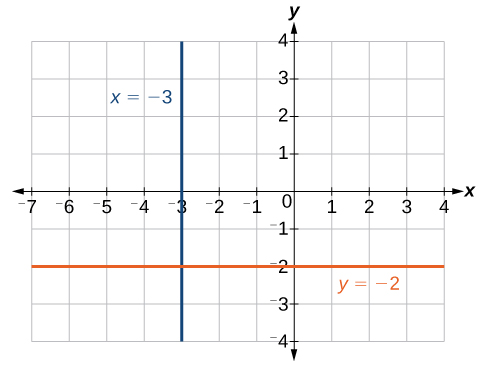
Suppose that we want to find the equation of a line containing the following points: \((−3,−5)\),\((−3,1)\),\((−3,3)\), and \((−3,5)\). First, we will find the slope.
Zero in the denominator means that the slope is undefined and, therefore, we cannot use the point-slope formula. However, we can plot the points. Notice that all of the \(x\)-coordinates are the same and we find a vertical line through \(x=−3\). See Figure \(\PageIndex{3}\).
The equation of a horizontal line is given as
\[y=c\]
where \(c\) is a constant. The slope of a horizontal line is zero, and for any \(x\)-value of a point on the line, the \(y\)-coordinate will be \(c\).
Suppose we want to find the equation of a line that contains the following set of points: \((−2,−2)\),\((0,−2)\),\((3,−2)\), and \((5,−2)\). We can use the point-slope formula. First, we find the slope using any two points on the line.
\[\begin{align*} m&= \dfrac{-2-(-2)}{0-(-2)}\\ &= \dfrac{0}{2}\\ &= 0 \end{align*}\]
Use any point for \((x_1,y_1)\) in the formula, or use the y-intercept.
\[\begin{align*} y-(-2)&= 0(x-3)\\ y+2&= 0\\ y&= -2 \end{align*}\]
The graph is a horizontal line through \(y=−2\). Notice that all of the y-coordinates are the same. See Figure \(\PageIndex{5}\).
Find the equation of the line passing through the given points: \((1,−3)\) and \((1,4)\).
Solution
The \(x\)-coordinate of both points is \(1\). Therefore, we have a vertical line, \(x=1\).
Determining Whether Graphs of Lines are Parallel or Perpendicular
Parallel lines have the same slope and different y-intercepts. Lines that are parallel to each other will never intersect. For example, Figure \(\PageIndex{6}\) shows the graphs of various lines with the same slope, \(m=2\).
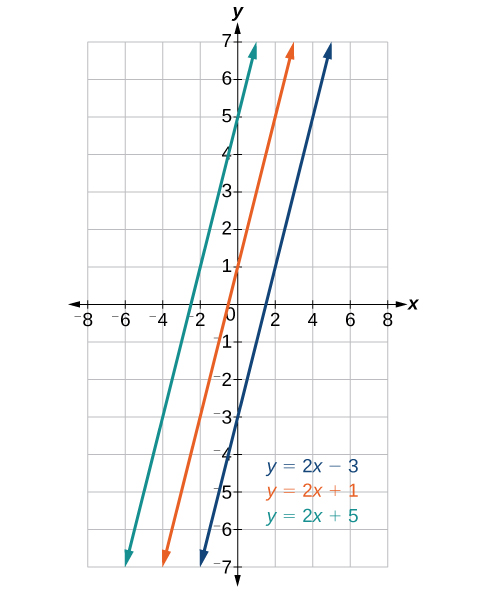
All of the lines shown in the graph are parallel because they have the same slope and different y-intercepts.
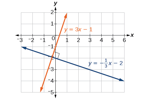
Lines that are perpendicular intersect to form a \(90^{\circ}\) -angle. The slope of one line is the negative reciprocal of the other. We can show that two lines are perpendicular if the product of the two slopes is \(−1:m_1⋅m_2=−1\). For example, Figure \(\PageIndex{7}\) shows the graph of two perpendicular lines. One line has a slope of \(3\); the other line has a slope of \(-\dfrac{1}{3}\).
\[\begin{align*} m_1\cdot m_2&= -1\\ 3\cdot \left (-\dfrac{1}{3} \right )&= -1\\ \end{align*}\]
Writing the Equations of Lines Parallel or Perpendicular to a Given Line
As we have learned, determining whether two lines are parallel or perpendicular is a matter of finding the slopes. To write the equation of a line parallel or perpendicular to another line, we follow the same principles as we do for finding the equation of any line. After finding the slope, use the point-slope formula to write the equation of the new line.
- Find the slope of the given line. The easiest way to do this is to write the equation in slope-intercept form.
- Use the slope and the given point with the point-slope formula.
- Simplify the line to slope-intercept form and compare the equation to the given line.
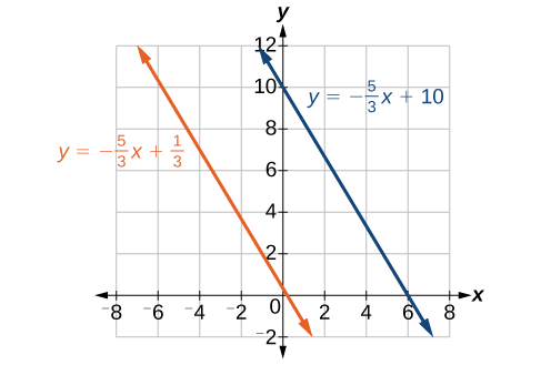
a. Write the equation of line parallel to a \(5x+3y=1\) and passing through the point \((3,5)\).
- Answer
-
First, we will write the equation in slope-intercept form to find the slope.
\[\begin{align*} 5x+3y&= 1\\ 3y&= -5x+1\\ y&= -\dfrac{5}{3}x+\dfrac{1}{3} \end{align*}\]
The slope is \(m=−\dfrac{5}{3}\). The y-intercept is \(13\), but that really does not enter into our problem, as the only thing we need for two lines to be parallel is the same slope. The one exception is that if the \(y\)-intercepts are the same, then the two lines are the same line. The next step is to use this slope and the given point with the point-slope formula.
\[\begin{align*} y-5&= -\dfrac{5}{3}(x-3)\\ y-5&= -\dfrac{5}{3}x+5\\ y&= -\dfrac{5}{3}x+10 \end{align*}\]
The equation of the line is \(y=−\dfrac{5}{3}x+10\). See Figure \(\PageIndex{6}\).
b. Find the equation of the line perpendicular to \(5x−3y+4=0\space(−4,1)\).
- Answer b
-
The first step is to write the equation in slope-intercept form.
\[\begin{align*} 5x-3y+4&= 0\\ -3y&= -5x-4\\ y&= \dfrac{5}{3}x+\dfrac{4}{3} \end{align*}\]
We see that the slope is \(m=\dfrac{5}{3}\). This means that the slope of the line perpendicular to the given line is the negative reciprocal, or \(-\dfrac{3}{5}\). Next, we use the point-slope formula with this new slope and the given point.
\[\begin{align*} y-1&= -\dfrac{3}{5}(x-(-4))\\ y-1&= -\dfrac{3}{5}x-\dfrac{12}{5}\\ y&= -\dfrac{3}{5}x-\dfrac{12}{5}+\dfrac{5}{5}\\ y&= -\dfrac{3}{5}x-\dfrac{7}{5} \end{align*}\]
Key Concepts
- A linear equation can be used to solve for an unknown in a number problem.
- Applications can be written as mathematical problems by identifying known quantities and assigning a variable to unknown quantities.
- Given two points, we can find the slope of a line using the slope formula.
- We can identify the slope and \(y\)-intercept of an equation in slope-intercept form.
- We can find the equation of a line given the slope and a point.
- We can also find the equation of a line given two points. Find the slope and use the point-slope formula.
- The standard form of a line has no fractions.
- Horizontal lines have a slope of zero and are defined as \(y=c\), where \(c\) is a constant.
- Vertical lines have an undefined slope (zero in the denominator), and are defined as \(x=c\), where \(c\) is a constant.
- Parallel lines have the same slope and different \(y\)-intercepts.