3.6: Absolute Value Functions
- Page ID
- 1496
\( \newcommand{\vecs}[1]{\overset { \scriptstyle \rightharpoonup} {\mathbf{#1}} } \)
\( \newcommand{\vecd}[1]{\overset{-\!-\!\rightharpoonup}{\vphantom{a}\smash {#1}}} \)
\( \newcommand{\dsum}{\displaystyle\sum\limits} \)
\( \newcommand{\dint}{\displaystyle\int\limits} \)
\( \newcommand{\dlim}{\displaystyle\lim\limits} \)
\( \newcommand{\id}{\mathrm{id}}\) \( \newcommand{\Span}{\mathrm{span}}\)
( \newcommand{\kernel}{\mathrm{null}\,}\) \( \newcommand{\range}{\mathrm{range}\,}\)
\( \newcommand{\RealPart}{\mathrm{Re}}\) \( \newcommand{\ImaginaryPart}{\mathrm{Im}}\)
\( \newcommand{\Argument}{\mathrm{Arg}}\) \( \newcommand{\norm}[1]{\| #1 \|}\)
\( \newcommand{\inner}[2]{\langle #1, #2 \rangle}\)
\( \newcommand{\Span}{\mathrm{span}}\)
\( \newcommand{\id}{\mathrm{id}}\)
\( \newcommand{\Span}{\mathrm{span}}\)
\( \newcommand{\kernel}{\mathrm{null}\,}\)
\( \newcommand{\range}{\mathrm{range}\,}\)
\( \newcommand{\RealPart}{\mathrm{Re}}\)
\( \newcommand{\ImaginaryPart}{\mathrm{Im}}\)
\( \newcommand{\Argument}{\mathrm{Arg}}\)
\( \newcommand{\norm}[1]{\| #1 \|}\)
\( \newcommand{\inner}[2]{\langle #1, #2 \rangle}\)
\( \newcommand{\Span}{\mathrm{span}}\) \( \newcommand{\AA}{\unicode[.8,0]{x212B}}\)
\( \newcommand{\vectorA}[1]{\vec{#1}} % arrow\)
\( \newcommand{\vectorAt}[1]{\vec{\text{#1}}} % arrow\)
\( \newcommand{\vectorB}[1]{\overset { \scriptstyle \rightharpoonup} {\mathbf{#1}} } \)
\( \newcommand{\vectorC}[1]{\textbf{#1}} \)
\( \newcommand{\vectorD}[1]{\overrightarrow{#1}} \)
\( \newcommand{\vectorDt}[1]{\overrightarrow{\text{#1}}} \)
\( \newcommand{\vectE}[1]{\overset{-\!-\!\rightharpoonup}{\vphantom{a}\smash{\mathbf {#1}}}} \)
\( \newcommand{\vecs}[1]{\overset { \scriptstyle \rightharpoonup} {\mathbf{#1}} } \)
\(\newcommand{\longvect}{\overrightarrow}\)
\( \newcommand{\vecd}[1]{\overset{-\!-\!\rightharpoonup}{\vphantom{a}\smash {#1}}} \)
\(\newcommand{\avec}{\mathbf a}\) \(\newcommand{\bvec}{\mathbf b}\) \(\newcommand{\cvec}{\mathbf c}\) \(\newcommand{\dvec}{\mathbf d}\) \(\newcommand{\dtil}{\widetilde{\mathbf d}}\) \(\newcommand{\evec}{\mathbf e}\) \(\newcommand{\fvec}{\mathbf f}\) \(\newcommand{\nvec}{\mathbf n}\) \(\newcommand{\pvec}{\mathbf p}\) \(\newcommand{\qvec}{\mathbf q}\) \(\newcommand{\svec}{\mathbf s}\) \(\newcommand{\tvec}{\mathbf t}\) \(\newcommand{\uvec}{\mathbf u}\) \(\newcommand{\vvec}{\mathbf v}\) \(\newcommand{\wvec}{\mathbf w}\) \(\newcommand{\xvec}{\mathbf x}\) \(\newcommand{\yvec}{\mathbf y}\) \(\newcommand{\zvec}{\mathbf z}\) \(\newcommand{\rvec}{\mathbf r}\) \(\newcommand{\mvec}{\mathbf m}\) \(\newcommand{\zerovec}{\mathbf 0}\) \(\newcommand{\onevec}{\mathbf 1}\) \(\newcommand{\real}{\mathbb R}\) \(\newcommand{\twovec}[2]{\left[\begin{array}{r}#1 \\ #2 \end{array}\right]}\) \(\newcommand{\ctwovec}[2]{\left[\begin{array}{c}#1 \\ #2 \end{array}\right]}\) \(\newcommand{\threevec}[3]{\left[\begin{array}{r}#1 \\ #2 \\ #3 \end{array}\right]}\) \(\newcommand{\cthreevec}[3]{\left[\begin{array}{c}#1 \\ #2 \\ #3 \end{array}\right]}\) \(\newcommand{\fourvec}[4]{\left[\begin{array}{r}#1 \\ #2 \\ #3 \\ #4 \end{array}\right]}\) \(\newcommand{\cfourvec}[4]{\left[\begin{array}{c}#1 \\ #2 \\ #3 \\ #4 \end{array}\right]}\) \(\newcommand{\fivevec}[5]{\left[\begin{array}{r}#1 \\ #2 \\ #3 \\ #4 \\ #5 \\ \end{array}\right]}\) \(\newcommand{\cfivevec}[5]{\left[\begin{array}{c}#1 \\ #2 \\ #3 \\ #4 \\ #5 \\ \end{array}\right]}\) \(\newcommand{\mattwo}[4]{\left[\begin{array}{rr}#1 \amp #2 \\ #3 \amp #4 \\ \end{array}\right]}\) \(\newcommand{\laspan}[1]{\text{Span}\{#1\}}\) \(\newcommand{\bcal}{\cal B}\) \(\newcommand{\ccal}{\cal C}\) \(\newcommand{\scal}{\cal S}\) \(\newcommand{\wcal}{\cal W}\) \(\newcommand{\ecal}{\cal E}\) \(\newcommand{\coords}[2]{\left\{#1\right\}_{#2}}\) \(\newcommand{\gray}[1]{\color{gray}{#1}}\) \(\newcommand{\lgray}[1]{\color{lightgray}{#1}}\) \(\newcommand{\rank}{\operatorname{rank}}\) \(\newcommand{\row}{\text{Row}}\) \(\newcommand{\col}{\text{Col}}\) \(\renewcommand{\row}{\text{Row}}\) \(\newcommand{\nul}{\text{Nul}}\) \(\newcommand{\var}{\text{Var}}\) \(\newcommand{\corr}{\text{corr}}\) \(\newcommand{\len}[1]{\left|#1\right|}\) \(\newcommand{\bbar}{\overline{\bvec}}\) \(\newcommand{\bhat}{\widehat{\bvec}}\) \(\newcommand{\bperp}{\bvec^\perp}\) \(\newcommand{\xhat}{\widehat{\xvec}}\) \(\newcommand{\vhat}{\widehat{\vvec}}\) \(\newcommand{\uhat}{\widehat{\uvec}}\) \(\newcommand{\what}{\widehat{\wvec}}\) \(\newcommand{\Sighat}{\widehat{\Sigma}}\) \(\newcommand{\lt}{<}\) \(\newcommand{\gt}{>}\) \(\newcommand{\amp}{&}\) \(\definecolor{fillinmathshade}{gray}{0.9}\)Learning Objectives
- Graph an absolute value function.
- Solve an absolute value equation.
Until the 1920s, the so-called spiral nebulae were believed to be clouds of dust and gas in our own galaxy, some tens of thousands of light years away. Then, astronomer Edwin Hubble proved that these objects are galaxies in their own right, at distances of millions of light years. Today, astronomers can detect galaxies that are billions of light years away. Distances in the universe can be measured in all directions. As such, it is useful to consider distance as an absolute value function. In this section, we will investigate absolute value functions.

Understanding Absolute Value
Recall that in its basic form \(f(x)=|x|\), the absolute value function, is one of our toolkit functions. The absolute value function is commonly thought of as providing the distance the number is from zero on a number line. Algebraically, for whatever the input value is, the output is the value without regard to sign.
Absolute Value Function
The absolute value function can be defined as a piecewise function
\[f(x)=|x|= \begin{cases} x & \text{ if }x{\geq}0 \\ -x & \text{ if } x<0 \end{cases}\]
Example \(\PageIndex{1}\): Determine a Number within a Prescribed Distance
Describe all values \(x\) within or including a distance of 4 from the number 5.
Solution
We want the distance between \(x\) and 5 to be less than or equal to 4. We can draw a number line, such as the one in , to represent the condition to be satisfied.

The distance from \(x\) to 5 can be represented using the absolute value as \(|x−5|\). We want the values of \(x\) that satisfy the condition \(| x−5 |\leq4\).
Analysis
Note that
\[\begin{align*} -4&{\leq}x-5 & x-5&\leq4 \\[4pt] 1&{\leq}x & x&{\leq}9 \end{align*}\]
So \(|x−5|\leq4\) is equivalent to \(1{\leq}x\leq9\).
However, mathematicians generally prefer absolute value notation.
Exercise \(\PageIndex{1}\)
Describe all values \(x\) within a distance of 3 from the number 2.
- Answer
-
\(|x−2|\leq3\)
Example \(\PageIndex{2}\): Resistance of a Resistor
Electrical parts, such as resistors and capacitors, come with specified values of their operating parameters: resistance, capacitance, etc. However, due to imprecision in manufacturing, the actual values of these parameters vary somewhat from piece to piece, even when they are supposed to be the same. The best that manufacturers can do is to try to guarantee that the variations will stay within a specified range, often ±1%, ±5%, or ±10%.
Suppose we have a resistor rated at 680 ohms, ±5%. Use the absolute value function to express the range of possible values of the actual resistance.
Solution
5% of 680 ohms is 34 ohms. The absolute value of the difference between the actual and nominal resistance should not exceed the stated variability, so, with the resistance \(R\) in ohms,
\[|R−680|\leq34 \nonumber\]
Exercise \(\PageIndex{2}\)
Students who score within 20 points of 80 will pass a test. Write this as a distance from 80 using absolute value notation.
- Answer
-
Using the variable \(p\) for passing, \(| p−80 |\leq20\)
Graphing an Absolute Value Function
The most significant feature of the absolute value graph is the corner point at which the graph changes direction. This point is shown at the origin in Figure \(\PageIndex{3}\).

Figure \(\PageIndex{3}\) shows the graph of \(y=2|x–3|+4\). The graph of \(y=|x|\) has been shifted right 3 units, vertically stretched by a factor of 2, and shifted up 4 units. This means that the corner point is located at \((3,4)\) for this transformed function.

Example \(\PageIndex{3}\): Writing an Equation for an Absolute Value Function
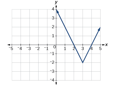
Write an equation for the function graphed in Figure \(\PageIndex{5}\).
Solution
The basic absolute value function changes direction at the origin, so this graph has been shifted to the right 3 units and down 2 units from the basic toolkit function. See Figure \(\PageIndex{6}\).
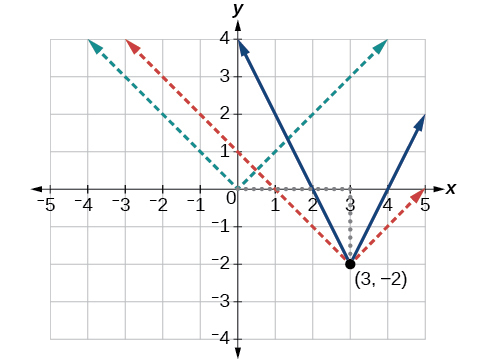
We also notice that the graph appears vertically stretched, because the width of the final graph on a horizontal line is not equal to 2 times the vertical distance from the corner to this line, as it would be for an unstretched absolute value function. Instead, the width is equal to 1 times the vertical distance as shown in Figure \(\PageIndex{7}\).
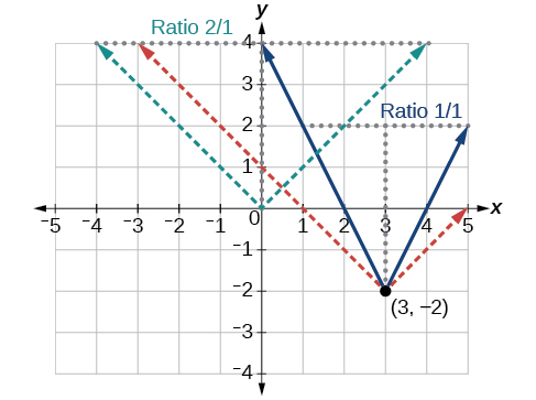
From this information we can write the equation
\[\begin{align*} f(x)&=2|x-3|-2, \;\;\;\;\;\; \text{treating the stretch as a vertial stretch, or} \\ f(x)&=|2(x-3)|-2, \;\;\; \text{treating the stretch as a horizontal compression.} \end{align*}\]
Analysis
Note that these equations are algebraically equivalent—the stretch for an absolute value function can be written interchangeably as a vertical or horizontal stretch or compression.
Q & A
If we couldn’t observe the stretch of the function from the graphs, could we algebraically determine it?
- Answer
-
Yes. If we are unable to determine the stretch based on the width of the graph, we can solve for the stretch factor by putting in a known pair of values for \(x\) and \(f(x)\).
\[f(x)=a|x−3|−2 \nonumber\]
Now substituting in the point \((1, 2)\)
\[\begin{align*} 2&=a|1-3|-2 \\ 4&=2a \\ a&=2 \end{align*}\]
Exercise \(\PageIndex{3}\)
Write the equation for the absolute value function that is horizontally shifted left 2 units, is vertically flipped, and vertically shifted up 3 units.
- Answer
-
\(f(x)=−| x+2 |+3\)
Q & A
Do the graphs of absolute value functions always intersect the vertical axis? The horizontal axis?
- Answer
-
Yes, they always intersect the vertical axis. The graph of an absolute value function will intersect the vertical axis when the input is zero.
No, they do not always intersect the horizontal axis. The graph may or may not intersect the horizontal axis, depending on how the graph has been shifted and reflected. It is possible for the absolute value function to intersect the horizontal axis at zero, one, or two points (Figure \(\PageIndex{8}\)).
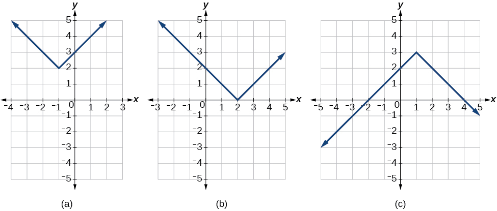
Figure \(\PageIndex{8}\): (a) The absolute value function does not intersect the horizontal axis. (b) The absolute value function intersects the horizontal axis at one point. (c) The absolute value function intersects the horizontal axis at two points.
Solving an Absolute Value Equation
Now that we can graph an absolute value function, we will learn how to solve an absolute value equation. To solve an equation such as \(8=|2x−6|\), we notice that the absolute value will be equal to 8 if the quantity inside the absolute value is 8 or -8. This leads to two different equations we can solve independently.
\[2x-6=8 \quad \text{ or } \quad 2x-6=-8 \nonumber\]
\[\begin{align*} 2x &= 14 & 2x &= -2 \\ x&=7 & x&=-1 \end{align*}\]
Knowing how to solve problems involving absolute value functions is useful. For example, we may need to identify numbers or points on a line that are at a specified distance from a given reference point.
An absolute value equation is an equation in which the unknown variable appears in absolute value bars. For example,
\[\begin{align*}|x|&=4, \nonumber \\[4pt] |2x−1| &=3, \\[4pt] |5x+2|−4 &=9. \end{align*}\]
Solutions to Absolute Value Equations
For real numbers \(A\) and \(B\), an equation of the form \(|A|=B\), with \(B\geq0\), will have solutions when \(A=B\) or \(A=−B\). If \(B<0\), the equation \(|A|=B\) has no solution.
How To ...
Given the formula for an absolute value function, find the horizontal intercepts of its graph.
- Isolate the absolute value term.
- Use \(|A|=B\) to write \(A=B\) or \(−A=B\), assuming \(B>0\).
- Solve for \(x\).
Example \(\PageIndex{4}\): Finding the Zeros of an Absolute Value Function
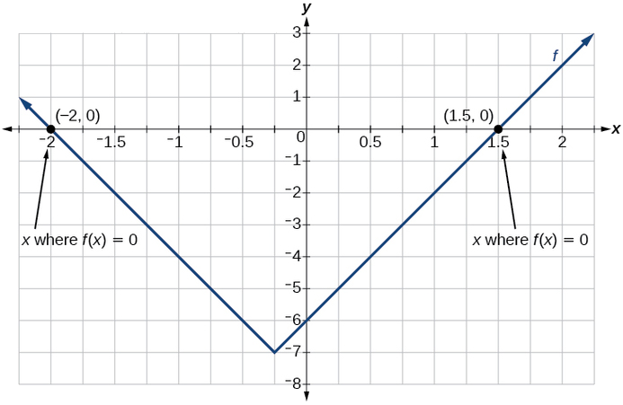
For the function \(f(x)=|4x+1|−7\), find the values of \(x\) such that \(f(x)=0\).
Solution
\[\begin{align*} 0&=|4x+1|-7 & & &\text{Substitute 0 for f(x).} \\ 7&=|4x+1| & & &\text{Isolate the absolute value on one side of the equation.} \\ 7&=4x+1 &\text{or} -7&=4x+1 &\text{Break into two separate equations and solve.} \\ 6&=4x & -8&=4x & \\ x&=\frac{6}{4}=1.5 & x&=\frac{-8}{4}=-2 \end{align*}\]
The function outputs 0 when \(x=1.5\) or \(x=−2\) (Figure \(\PageIndex{9}\)).
Exercise \(\PageIndex{4}\)
For the function \(f(x)=|2x−1|−3\), find the values of \(x\) such that \(f(x)=0\).
Solution
\(x=−1\) or \(x=2\)
Q & A
Should we always expect two answers when solving \(|A|=B\)?
Answer
No. We may find one, two, or even no answers. For example, there is no solution to \(2+|3x−5|=1\).
How To ...
Given an absolute value equation, solve it.
- Isolate the absolute value term.
- Use \(|A|=B\) to write \(A=B\) or \(A=−B\).
- Solve for \(x\).
Example \(\PageIndex{5}\): Solving an Absolute Value Equation
Solve \(1=4|x−2|+2\).
Solution
Isolating the absolute value on one side of the equation gives the following.
\[\begin{align*} 1&=4|x-2|+2 \\ -1&=4|x-2| \\ -\frac{1}{4}&=|x-2| \end{align*}\]
The absolute value always returns a positive value, so it is impossible for the absolute value to equal a negative value. At this point, we notice that this equation has no solutions.
Q & A
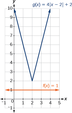
In Example \(\PageIndex{5}\), if \(f(x)=1\) and \(g(x)=4|x−2|+2\) were graphed on the same set of axes, would the graphs intersect?
Answer
No. The graphs of \(f\) and \(g\) would not intersect, as shown in Figure \(\PageIndex{10}\). This confirms, graphically, that the equation \(1=4|x−2|+2\) has no solution.
Find where the graph of the function \(f(x)=−| x+2 |+3\) intersects the horizontal and vertical axes.
\(f(0)=1\), so the graph intersects the vertical axis at \((0,1)\). \(f(x)=0\) when \(x=−5\) and \(x=1\) so the graph intersects the horizontal axis at \((−5,0)\) and \((1,0)\).
Solving an Absolute Value Inequality
Absolute value equations may not always involve equalities. Instead, we may need to solve an equation within a range of values. We would use an absolute value inequality to solve such an equation. An absolute value inequality is an equation of the form
\[|A|<B,\;|A|{\leq}B,|A|>B, \nonumber\]
or
\[ |A|{\geq}B, \nonumber\]
where an expression \(A\) (and possibly but not usually \(B\)) depends on a variable \(x\). Solving the inequality means finding the set of all \(x\) that satisfy the inequality. Usually this set will be an interval or the union of two intervals.
There are two basic approaches to solving absolute value inequalities: graphical and algebraic. The advantage of the graphical approach is we can read the solution by interpreting the graphs of two functions. The advantage of the algebraic approach is it yields solutions that may be difficult to read from the graph.
For example, we know that all numbers within 200 units of 0 may be expressed as
\[|x|<200 \nonumber\]
or
\[ −200<x<200 \nonumber\]
Suppose we want to know all possible returns on an investment if we could earn some amount of money within $200 of $600. We can solve algebraically for the set of values \(x\) such that the distance between \(x\) and 600 is less than 200. We represent the distance between \(x\) and 600 as \(|x−600|\).
\[|x−600|<200\]
or
\[−200<x−600<200\]
\[\begin{align*} −200+600< &x−600+600<200+600 \\[4pt] 400< &x<800 \end{align*}\]
This means our returns would be between $400 and $800.
Sometimes an absolute value inequality problem will be presented to us in terms of a shifted and/or stretched or compressed absolute value function, where we must determine for which values of the input the function’s output will be negative or positive.
How To ...
Given an absolute value inequality of the form \(|x−A|{\leq}B\) for real numbers \(a\) and \(b\) where \(b\) is positive, solve the absolute value inequality algebraically.
- Find boundary points by solving \(|x−A|=B\).
- Test intervals created by the boundary points to determine where \(|x−A|{\leq}B\).
- Write the interval or union of intervals satisfying the inequality in interval, inequality, or set-builder notation.
Example \(\PageIndex{6}\): Solving an Absolute Value Inequality
Solve \(|x −5|{\leq}4\).
Solution
With both approaches, we will need to know first where the corresponding equality is true. In this case we first will find where \(|x−5|=4\). We do this because the absolute value is a function with no breaks, so the only way the function values can switch from being less than 4 to being greater than 4 is by passing through where the values equal 4. Solve \(|x−5|=4\).
\[\begin{align*} x−5&=4 &\text{ or }\;\;\;\;\;\;\;\; x&=9 \\ x−5&=−4 & x&=1\end{align*}\]
After determining that the absolute value is equal to 4 at \(x=1\) and \(x=9\), we know the graph can change only from being less than 4 to greater than 4 at these values. This divides the number line up into three intervals:
\[x<1,\; 1<x<9, \text{ and } x>9. \nonumber\]
To determine when the function is less than 4, we could choose a value in each interval and see if the output is less than or greater than 4, as shown in Table \(\PageIndex{1}\).
| Interval test \(x\) | \(f(x)\) | \(<4\) or \(>4\) | |
|---|---|---|---|
| \(x<1\) | 0 | \(|0-5|=5\) | Greater than |
| \(1<x<9\) | 6 | \(|6-5|=1\) | Less than |
| \(x>9\) | 11 | \(|11-5|=6\) | Greater than |
Because \(1{\leq}x{\leq}9\) is the only interval in which the output at the test value is less than 4, we can conclude that the solution to \(|x−5|{\leq}4\) is \(1{\leq}x{\leq}9\), or \([1,9]\).
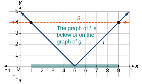
To use a graph, we can sketch the function \(f(x)=|x−5|\). To help us see where the outputs are 4, the line \(g(x)=4\) could also be sketched as in Figure \(\PageIndex{11}\).
We can see the following:
- The output values of the absolute value are equal to 4 at \(x=1\) and \(x=9\).
- The graph of \(f\) is below the graph of \(g\) on \(1<x<9\). This means the output values of \(f(x)\) are less than the output values of \(g(x)\).
- The absolute value is less than or equal to 4 between these two points, when \(1{\leq}x\leq9\). In interval notation, this would be the interval \([1,9]\).
Analysis
For absolute value inequalities,
\[|x−A|<C,\;\;\;\;\;\;\;\;\;\;\;\;\;\;\; |x−A|>C, \\−C<x−A<C,\;\;\;\; x−A<−C \text{ or } x−A>C. \nonumber\]
The \(<\) or \(>\) symbol may be replaced by \(\leq\) or \(\geq\).
So, for this example, we could use this alternative approach.
\[\begin{align*} |x−5|&{\leq}4 \\ −4&{\leq}x−5{\leq}4 &\text{Rewrite by removing the absolute value bars.} \\ −4+5&{\leq}x−5+5{\leq}4+5 &\text{Isolate the x.} \\ 1&{\leq}x\leq9 \end{align*}\]
Exercise \(\PageIndex{5}\)
Solve \(|x+2| \leq 6\).
- Answer
-
\(-8 \leq x \leq 4\)
How To ...
Given an absolute value function, solve for the set of inputs where the output is positive (or negative).
- Set the function equal to zero, and solve for the boundary points of the solution set.
- Use test points or a graph to determine where the function’s output is positive or negative.
Example \(\PageIndex{7}\): Using a Graphical Approach to Solve Absolute Value Inequalities
Given the function \(f(x)=−\frac{1}{2}|4x−5|+3\), determine the \(x\)-values for which the function values are negative.
Solution
We are trying to determine where \(f(x)<0\), which is when \(−\frac{1}{2}|4x−5|+3<0\). We begin by isolating the absolute value.
\[ \begin{align*} -\frac{1}{2}|4x−5|&<−3 \;\;\; \text{Multiply both sides by –2, and reverse the inequality.} \\ |4x−5|&>6\end{align*}\]
Next we solve for the equality \(|4x−5|=6\).
\[\begin{align*} 4x-5&=6 & 4x-5&=-6 \\ 4x-6&=6 \end{align*}\]
or
\[\begin{align*} 4x&=-1 \\ x&=\frac{11}{4} & x&=-\frac{1}{4} \end{align*}\]
Now, we can examine the graph of \(f\) to observe where the output is negative. We will observe where the branches are below the \(x\)-axis. Notice that it is not even important exactly what the graph looks like, as long as we know that it crosses the horizontal axis at \(x=−\frac{1}{4}\) and \(x=\frac{11}{4}\) and that the graph has been reflected vertically. See Figure \(\PageIndex{12}\).
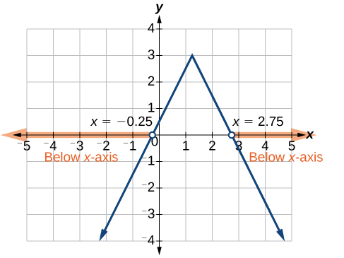
We observe that the graph of the function is below the \(x\)-axis left of \(x=−\frac{1}{4}\) and right of \(x=\frac{11}{4}\). This means the function values are negative to the left of the first horizontal intercept at \(x=−\frac{1}{4}\), and negative to the right of the second intercept at \(x=\frac{11}{4} \). This gives us the solution to the inequality.
\[x<−\frac{1}{4} \text{ or } x>1\frac{1}{4} \nonumber\]
In interval notation, this would be \(( −\infty,−0.25 )\cup( 2.75,\infty)\).
Exercise \(\PageIndex{6}\)
Solve \(−2|k−4|\leq−6\).
- Answer
-
\(k\leq1\) or \(k\geq7\); in interval notation, this would be \(\left(−\infty,1\right]\cup\left[7,\infty\right)\)
Key Concepts
- The absolute value function is commonly used to measure distances between points.
- Applied problems, such as ranges of possible values, can also be solved using the absolute value function.
- The graph of the absolute value function resembles a letter V. It has a corner point at which the graph changes direction.
- In an absolute value equation, an unknown variable is the input of an absolute value function.
- If the absolute value of an expression is set equal to a positive number, expect two solutions for the unknown variable.
- An absolute value equation may have one solution, two solutions, or no solutions.
- An absolute value inequality is similar to an absolute value equation but takes the form | A |<B, | A |≤B, | A |>B, or | A |≥B.It can be solved by determining the boundaries of the solution set and then testing which segments are in the set.
- Absolute value inequalities can also be solved graphically.
Glossary
absolute value equation
an equation of the form \(|A|=B\), with \(B\geq0\); it will have solutions when \(A=B\) or \(A=−B\)
absolute value inequality
a relationship in the form \(|A|<B\), \(|A|{\leq}B\), \(|A|>B\), or \(|A|{\geq}B\)


