
2.2: Linear Functions and Their Graphs
- Page ID
- 6234
\( \newcommand{\vecs}[1]{\overset { \scriptstyle \rightharpoonup} {\mathbf{#1}} } \)
\( \newcommand{\vecd}[1]{\overset{-\!-\!\rightharpoonup}{\vphantom{a}\smash {#1}}} \)
\( \newcommand{\dsum}{\displaystyle\sum\limits} \)
\( \newcommand{\dint}{\displaystyle\int\limits} \)
\( \newcommand{\dlim}{\displaystyle\lim\limits} \)
\( \newcommand{\id}{\mathrm{id}}\) \( \newcommand{\Span}{\mathrm{span}}\)
( \newcommand{\kernel}{\mathrm{null}\,}\) \( \newcommand{\range}{\mathrm{range}\,}\)
\( \newcommand{\RealPart}{\mathrm{Re}}\) \( \newcommand{\ImaginaryPart}{\mathrm{Im}}\)
\( \newcommand{\Argument}{\mathrm{Arg}}\) \( \newcommand{\norm}[1]{\| #1 \|}\)
\( \newcommand{\inner}[2]{\langle #1, #2 \rangle}\)
\( \newcommand{\Span}{\mathrm{span}}\)
\( \newcommand{\id}{\mathrm{id}}\)
\( \newcommand{\Span}{\mathrm{span}}\)
\( \newcommand{\kernel}{\mathrm{null}\,}\)
\( \newcommand{\range}{\mathrm{range}\,}\)
\( \newcommand{\RealPart}{\mathrm{Re}}\)
\( \newcommand{\ImaginaryPart}{\mathrm{Im}}\)
\( \newcommand{\Argument}{\mathrm{Arg}}\)
\( \newcommand{\norm}[1]{\| #1 \|}\)
\( \newcommand{\inner}[2]{\langle #1, #2 \rangle}\)
\( \newcommand{\Span}{\mathrm{span}}\) \( \newcommand{\AA}{\unicode[.8,0]{x212B}}\)
\( \newcommand{\vectorA}[1]{\vec{#1}} % arrow\)
\( \newcommand{\vectorAt}[1]{\vec{\text{#1}}} % arrow\)
\( \newcommand{\vectorB}[1]{\overset { \scriptstyle \rightharpoonup} {\mathbf{#1}} } \)
\( \newcommand{\vectorC}[1]{\textbf{#1}} \)
\( \newcommand{\vectorD}[1]{\overrightarrow{#1}} \)
\( \newcommand{\vectorDt}[1]{\overrightarrow{\text{#1}}} \)
\( \newcommand{\vectE}[1]{\overset{-\!-\!\rightharpoonup}{\vphantom{a}\smash{\mathbf {#1}}}} \)
\( \newcommand{\vecs}[1]{\overset { \scriptstyle \rightharpoonup} {\mathbf{#1}} } \)
\(\newcommand{\longvect}{\overrightarrow}\)
\( \newcommand{\vecd}[1]{\overset{-\!-\!\rightharpoonup}{\vphantom{a}\smash {#1}}} \)
\(\newcommand{\avec}{\mathbf a}\) \(\newcommand{\bvec}{\mathbf b}\) \(\newcommand{\cvec}{\mathbf c}\) \(\newcommand{\dvec}{\mathbf d}\) \(\newcommand{\dtil}{\widetilde{\mathbf d}}\) \(\newcommand{\evec}{\mathbf e}\) \(\newcommand{\fvec}{\mathbf f}\) \(\newcommand{\nvec}{\mathbf n}\) \(\newcommand{\pvec}{\mathbf p}\) \(\newcommand{\qvec}{\mathbf q}\) \(\newcommand{\svec}{\mathbf s}\) \(\newcommand{\tvec}{\mathbf t}\) \(\newcommand{\uvec}{\mathbf u}\) \(\newcommand{\vvec}{\mathbf v}\) \(\newcommand{\wvec}{\mathbf w}\) \(\newcommand{\xvec}{\mathbf x}\) \(\newcommand{\yvec}{\mathbf y}\) \(\newcommand{\zvec}{\mathbf z}\) \(\newcommand{\rvec}{\mathbf r}\) \(\newcommand{\mvec}{\mathbf m}\) \(\newcommand{\zerovec}{\mathbf 0}\) \(\newcommand{\onevec}{\mathbf 1}\) \(\newcommand{\real}{\mathbb R}\) \(\newcommand{\twovec}[2]{\left[\begin{array}{r}#1 \\ #2 \end{array}\right]}\) \(\newcommand{\ctwovec}[2]{\left[\begin{array}{c}#1 \\ #2 \end{array}\right]}\) \(\newcommand{\threevec}[3]{\left[\begin{array}{r}#1 \\ #2 \\ #3 \end{array}\right]}\) \(\newcommand{\cthreevec}[3]{\left[\begin{array}{c}#1 \\ #2 \\ #3 \end{array}\right]}\) \(\newcommand{\fourvec}[4]{\left[\begin{array}{r}#1 \\ #2 \\ #3 \\ #4 \end{array}\right]}\) \(\newcommand{\cfourvec}[4]{\left[\begin{array}{c}#1 \\ #2 \\ #3 \\ #4 \end{array}\right]}\) \(\newcommand{\fivevec}[5]{\left[\begin{array}{r}#1 \\ #2 \\ #3 \\ #4 \\ #5 \\ \end{array}\right]}\) \(\newcommand{\cfivevec}[5]{\left[\begin{array}{c}#1 \\ #2 \\ #3 \\ #4 \\ #5 \\ \end{array}\right]}\) \(\newcommand{\mattwo}[4]{\left[\begin{array}{rr}#1 \amp #2 \\ #3 \amp #4 \\ \end{array}\right]}\) \(\newcommand{\laspan}[1]{\text{Span}\{#1\}}\) \(\newcommand{\bcal}{\cal B}\) \(\newcommand{\ccal}{\cal C}\) \(\newcommand{\scal}{\cal S}\) \(\newcommand{\wcal}{\cal W}\) \(\newcommand{\ecal}{\cal E}\) \(\newcommand{\coords}[2]{\left\{#1\right\}_{#2}}\) \(\newcommand{\gray}[1]{\color{gray}{#1}}\) \(\newcommand{\lgray}[1]{\color{lightgray}{#1}}\) \(\newcommand{\rank}{\operatorname{rank}}\) \(\newcommand{\row}{\text{Row}}\) \(\newcommand{\col}{\text{Col}}\) \(\renewcommand{\row}{\text{Row}}\) \(\newcommand{\nul}{\text{Nul}}\) \(\newcommand{\var}{\text{Var}}\) \(\newcommand{\corr}{\text{corr}}\) \(\newcommand{\len}[1]{\left|#1\right|}\) \(\newcommand{\bbar}{\overline{\bvec}}\) \(\newcommand{\bhat}{\widehat{\bvec}}\) \(\newcommand{\bperp}{\bvec^\perp}\) \(\newcommand{\xhat}{\widehat{\xvec}}\) \(\newcommand{\vhat}{\widehat{\vvec}}\) \(\newcommand{\uhat}{\widehat{\uvec}}\) \(\newcommand{\what}{\widehat{\wvec}}\) \(\newcommand{\Sighat}{\widehat{\Sigma}}\) \(\newcommand{\lt}{<}\) \(\newcommand{\gt}{>}\) \(\newcommand{\amp}{&}\) \(\definecolor{fillinmathshade}{gray}{0.9}\)Learning Objectives
- Graph a line by plotting points.
- Determine the slope of a line.
- Identify and graph a linear function using the slope and \(y\)-intercept.
- Interpret solutions to linear equations and inequalities graphically.
A Review of Graphing Lines
Recall that the set of all solutions to a linear equation can be represented on a rectangular coordinate plane using a straight line through at least two points; this line is called its graph. For example, to graph the linear equation \(8x + 4y = 12\) we would first solve for \(y\).
\(\begin{aligned} 8 x + 4 y & = 12 \quad\quad\quad\quad \color{Cerulean}{Subtract\: 8x\: on\: both\: sides.} \\ 4 y & = - 8 x + 12 \quad \color{Cerulean}{Divide\: both\: sides\: by\: 4.} \\ y & = \frac { - 8 x + 12 } { 4 }\quad \color{Cerulean}{Simplify.} \\ y & = \frac { - 8 x } { 4 } + \frac { 12 } { 4 } \\ y & = - 2 x + 3 \end{aligned}\)
Written in this form, we can see that \(y\) depends on \(x\); in other words, \(x\) is the independent variable18 and \(y\) is the dependent variable19. Choose at least two \(x\)-values and find the corresponding \(y\)-values. It is a good practice to choose zero, some negative numbers, as well as some positive numbers. Here we will choose five \(x\)-values, determine the corresponding \(y\)-values, and then form a representative set of ordered pair solutions.
| \(x\) | \(y\) | \(y=-2x+3\) | Solutions |
|---|---|---|---|
|
\(−2\) |
\(7\) |
\(y=−2(\color{Cerulean}{−2}\color{Black}{)}+3=4+3=7\) |
\((−2, 7)\) |
|
\(−1\) |
\(5\) |
\(y=−2(\color{Cerulean}{−1}\color{Black}{)}+3=2+3=5\) |
\((−1, 5)\) |
|
\(0\) |
\(3\) |
\(y=−2(\color{Cerulean}{0}\color{Black}{)}+3=0+3=3\) |
\((0, 3)\) |
|
\(4\) |
\(−5\) |
\(y=−2(\color{Cerulean}{4}\color{Black}{)}+3=−8+3=−5\) |
\((4, −5)\) |
|
\(6\) |
\(−9\) |
\(y=−2(\color{Cerulean}{6}\color{Black}{)}+3=−12+3=−9\) |
\((6, −9)\) |
Plot the points and draw a line through the points with a straightedge. Be sure to add arrows on either end to indicate that the graph extends indefinitely.
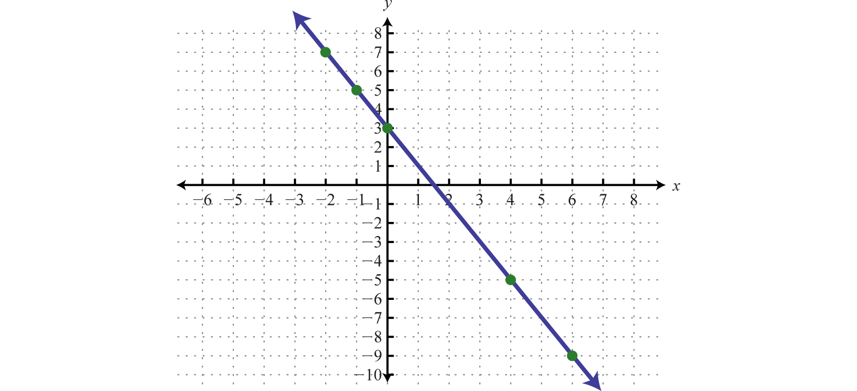
The resulting line represents all solutions to \(8x+4y=12\), of which there are infinitely many. The above process describes the technique for graphing known as plotting points20. This technique will be used to graph more complicated functions as we progress in this course.
The steepness of any incline can be measured as the ratio of the vertical change to the horizontal change. For example, a \(5\)% incline can be written as \(\frac{5}{100}\), which means that for every \(100\) feet forward, the height increases \(5\) feet.

In mathematics, we call the incline of a line the slope21, denoted by the letter m. The vertical change is called the rise22 and the horizontal change is called the run23. Given any two points \((x1, y1)\) and \((x2, y2)\), we can obtain the rise and run by subtracting the corresponding coordinates.

This leads us to the slope formula24. Given any two points \((x1, y1)\) and \((x2, y2)\), the slope is given by:
\(\color{Cerulean}{Slope} \:\:\:\color{Black}{m} = \frac {rise} {run} = \frac { y _ { 2 } - y _ { 1 } } { x _ { 2 } - x _ { 1 } } = \frac { \Delta y } { \Delta x } \quad \begin{array} { l l } { \color{Cerulean} { \gets\:\: Change\: in\: } y } \\ { \color{Cerulean} {\gets\:\: Change\: in\: } x } \end{array}\)
The Greek letter delta (\(Δ\)) is often used to describe the change in a quantity. Therefore, the slope is sometimes described using the notation \(\frac{Δy}{Δx}\), which represents the change in \(y\) divided by the change in \(x\).
Example \(\PageIndex{1}\):
Find the slope of the line passing through \((−3, −5)\) and \((2, 1)\).
Solution
Given \((−3, −5)\) and \((2, 1)\), calculate the difference of the \(y\)-values divided by the difference of the x-values. Take care to be consistent when subtracting the coordinates:
\(\begin{array} { l l } { \left( x _ { 1 } , y _ { 1 } \right) } & { \left( x _ { 2 } , y _ { 2 } \right) } \\ { ( - 3 , - 5 ) } & { ( 2,1 ) } \end{array}\)
\(\begin{aligned} m & = \frac { y _ { 2 } - y _ { 1 } } { x _ { 2 } - x _ { 1 } } \\ & = \frac { 1 - ( - 5 ) } { 2 - ( - 3 ) } \\ & = \frac { 1 + 5 } { 2 + 3 } \\ & = \frac { 6 } { 5 } \end{aligned}\)
It does not matter which point you consider to be the first and second. However, because subtraction is not commutative, you must take care to subtract the coordinates of the first point from the coordinates of the second point in the same order. For example, we obtain the same result if we apply the slope formula with the points switched:
\(\begin{array} { l } { \left( x _ { 1 } , y _ { 1 } \right) \quad \left( x _ { 2 } , y _ { 2 } \right) } \\ { ( 2,1 ) \quad ( - 3 , - 5 ) } \end{array}\)
\(\begin{aligned} m & = \frac { y _ { 2 } - y _ { 1 } } { x _ { 2 } - x _ { 1 } } \\ & = \frac { - 5 - 1 } { - 3 - 2 } \\ & = \frac { - 6 } { - 5 } \\ & = \frac { 6 } { 5 } \end{aligned}\)
Answer:
\(m=\frac{6}{5}\)
Verify that the slope is \(\frac{6}{5}\) by graphing the line described in the previous example.
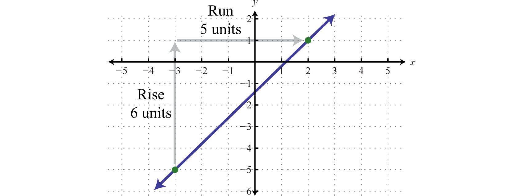
Certainly the graph is optional; the beauty of the slope formula is that, given any two points, we can obtain the slope using only algebra.
Example \(\PageIndex{2}\):
Find the \(y\)-value for which the slope of the line passing through \((6, −3)\) and \((−9, y)\) is \(−\frac{2}{3}\).
Solution
Substitute the given information into the slope formula.
\(\begin{array} { l l } { \text { Slope } } & { \left( x _ { 1 } , y _ { 1 } \right) } & { \left( x _ { 2 } , y _ { 2 } \right) } \\ { m = - \frac { 2 } { 3 } } & { ( 6 , - 3 ) } & { ( - 9 , y ) } \end{array}\)
\(\begin{aligned} m & = \frac { y _ { 2 } - y _ { 1 } } { x _ { 2 } - x _ { 1 } } \\ - \frac { 2 } { 3 } & = \frac { y - ( - 3 ) } { - 9 - 6 } \\ - \frac { 2 } { 3 } & = \frac { y + 3 } { - 15 } \end{aligned}\)
After substituting in the given information, the only variable left is \(y\). Solve.
\(\begin{aligned} \color{Cerulean}{- 15}\color{Black}{ \left( - \frac { 2 } { 3 } \right)} & = \color{Cerulean}{- 15}\color{Black}{ \left( - \frac { y + 3 } { 15 } \right)} \\ 10 & = y + 3 \\ 7 & = y \end{aligned}\)
Answer:
\(y=7\)
There are four geometric cases for the value of the slope.

Reading the graph from left to right, lines with an upward incline have positive slopes and lines with a downward incline have negative slopes. The other two cases involve horizontal and vertical lines. Recall that if \(k\) is a real number we have
\(\begin{array} { l } { y = k \color{Cerulean} { Horizontal line } } \\ { x = k \color{Cerulean} { Vertical line } } \end{array}\)
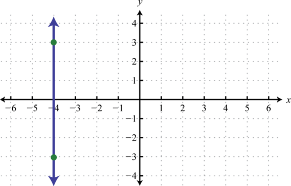
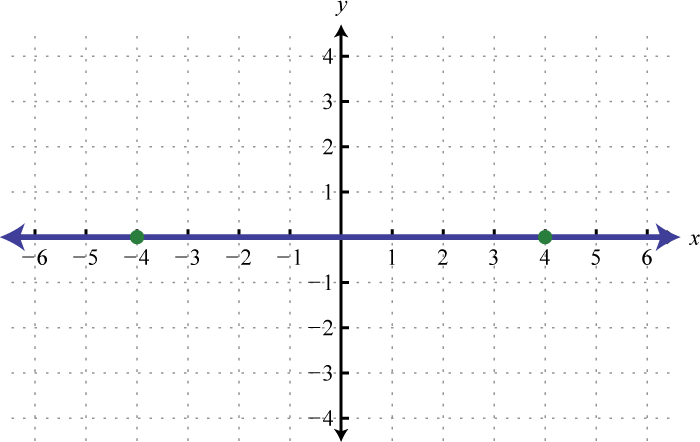
For example, if we graph \(y=2\) we obtain a horizontal line, and if we graph \(x=−4\) we obtain a vertical line.
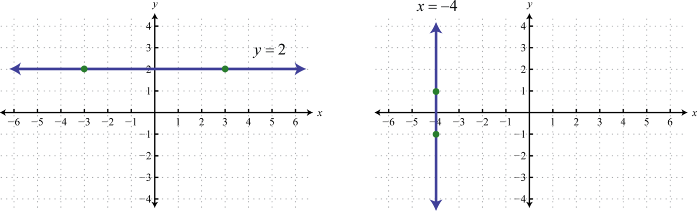
From the graphs we can determine two points and calculate the slope using the slope formula.
| Horizontal Line | Vertical Line |
|---|---|
|
\(\begin{array} { l l } { \left( x _ { 1 } , y _ { 1 } \right) } & { \left( x _ { 2 } , y _ { 2 } \right) } \\ { ( - 3,2 ) } & { ( 3,2 ) } \end{array}\) \(\begin{aligned} m & = \frac { y _ { 2 } - y _ { 1 } } { x _ { 2 } - x _ { 1 } } \\ & = \frac { 2 - ( 2 ) } { 3 - ( - 3 ) } \\ & = \frac { 2 - 2 } { 3 + 3 } \\ & = \frac { 0 } { 6 } = 0 \end{aligned}\) |
\(\begin{array} { c c } { \left( x _ { 1 } , y _ { 1 } \right) } & { \left( x _ { 2 } , y _ { 2 } \right) } \\ { ( - 4 , - 1 ) } & { ( - 4,1 ) } \end{array}\) \(\begin{aligned} m & = \frac { y _ { 2 } - y _ { 1 } } { x _ { 2 } - x _ { 1 } } \\ & = \frac { 1 - ( - 1 ) } { - 4 - ( - 4 ) } \\ & = \frac { 1 + 1 } { - 4 + 4 } \\ & = \frac { 2 } { 0 } \quad\quad\quad\quad \color{Cerulean} { Undefined } \end{aligned}\) |
Notice that the points on the horizontal line share the same \(y\)-values. Therefore, the rise is zero and hence the slope is zero. The points on the vertical line share the same \(x\)-values. Consequently, the run is zero, leading to an undefined slope. In general,

Linear Functions
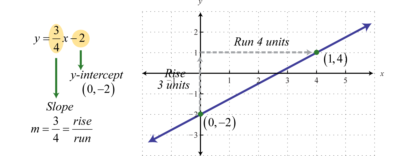
Given any linear equation in standard form25, \(ax + by = c\), we can solve for \(y\) to obtain slope-intercept form26, \(y = mx + b\). For example,
\(\begin{aligned} 3 x - 4 y & = 8\quad\quad\quad\color{Cerulean}{\gets \:\:Standard\: form} \\ - 4 y & = - 3 x + 8 \\ y & = \frac { - 3 x + 8 } { - 4 } \\ y & = \frac { - 3 x } { - 4 } + \frac { 8 } { - 4 } \\ y & = \frac { 3 } { 4 } x - 2 \quad\color{Cerulean} {\gets\:\: Slope-lntercept\: Form } \end{aligned}\)
Where \(x=0\), we can see that \(y=−2\) and thus \((0,−2)\) is an ordered pair solution. This is the point where the graph intersects the \(y\)-axis and is called the \(y\)-intercept27. We can use this point and the slope as a means to quickly graph a line. For example, to graph \(y=\frac{3}{4}x−2\), start at the \(y\)-intercept \((0,−2)\) and mark off the slope to find a second point. Then use these points to graph the line as follows:
The vertical line test indicates that this graph represents a function. Furthermore, the domain and range consists of all real numbers.
In general, a linear function28 is a function that can be written in the form
\(f ( x ) = m x + b\:\:\color{Cerulean}{Linear\:Function}\)
where the slope \(m\) and \(b\) represent any real numbers. Because \(y = f (x)\), we can use \(y\) and \(f (x)\) interchangeably, and ordered pair solutions on the graph \((x, y)\) can be written in the form \((x, f (x))\).
\(( x , y ) \quad \color{Cerulean}{\Leftrightarrow} \quad \color{Black}{(} x , f ( x ) )\)
We know that any \(y\)-intercept will have an \(x\)-value equal to zero. Therefore, the \(y\)-intercept can be expressed as the ordered pair \((0, f (0))\).For linear functions,
\(\begin{aligned} f ( \color{Cerulean}{0}\color{Black}{ )} & = m ( \color{Cerulean}{0}\color{Black}{ )} + b \\ & = b \end{aligned}\)
Hence, the \(y\)-intercept of any linear function is \((0, b)\).To find the x-intercept29, the point where the function intersects the \(x\)-axis, we find \(x\) where \(y = 0\) or \(f (x) = 0\).
Example \(\PageIndex{3}\):
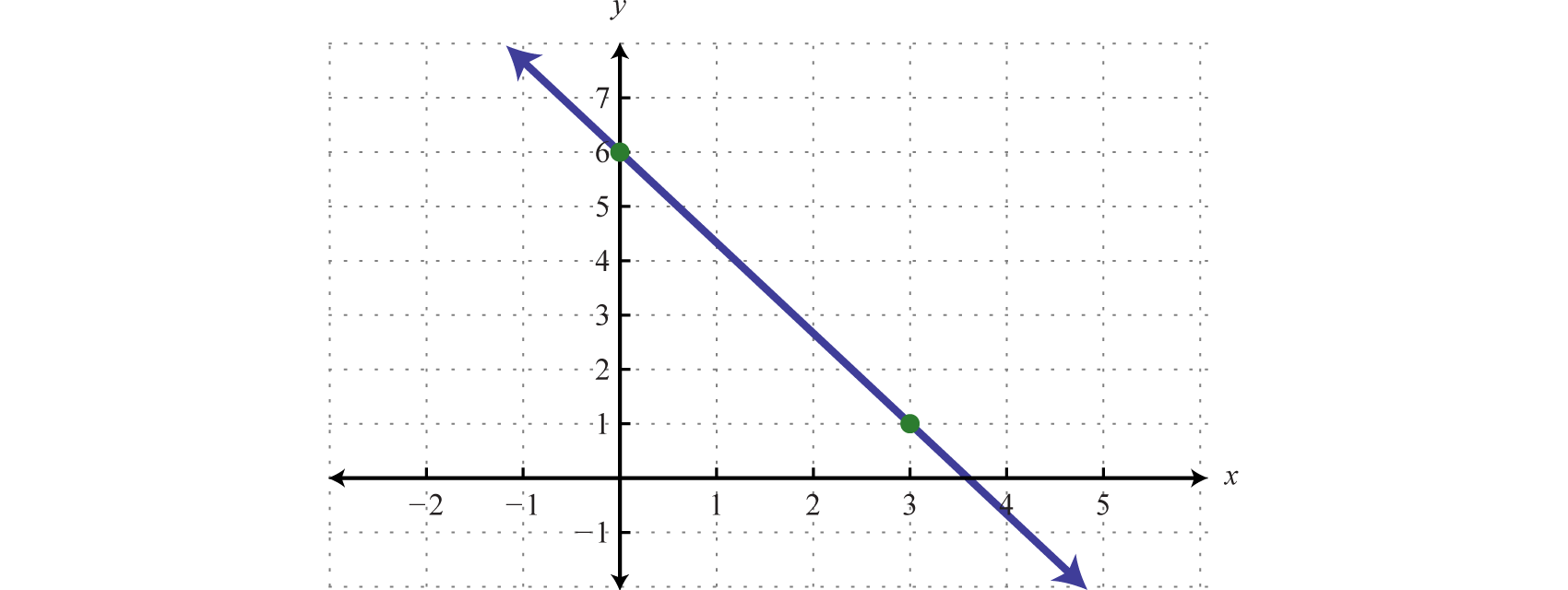
Graph the linear function \(f(x)=−\frac{5}{3}x+6\) and label the \(x\)-intercept.
Solution
From the function, we see that \(f(0)=6\) (or \(b=6\)) and thus the \(y\)-intercept is \((0, 6)\). Also, we can see that the slope \(m=−\frac{5}{3}=−\frac{5}{3}=\frac{rise}{run}\). Starting from the \(y\)-intercept, mark a second point down \(5\) units and right \(3\) units. Draw the line passing through these two points with a straightedge.
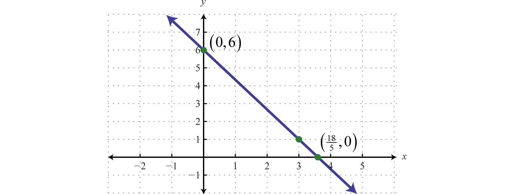
To determine the \(x\)-intercept, find the \(x\)-value where the function is equal to zero. In other words, determine \(x\) where \(f(x)=0\).
\(\begin{aligned} f ( x ) & = - \frac { 5 } { 3 } x + 6 \\ 0 & = - \frac { 5 } { 3 } x + 6 \\ \frac { 5 } { 3 } x & = 6 \\ \left( \color{Cerulean}{\frac { 3 } { 5 }} \right) \frac { 5 } { 3 } x & = \left( \color{Cerulean}{\frac { 3 } { 5 }} \right) 6 \\ x & = \frac { 18 } { 5 } = 3 \frac { 3 } { 5 } \end{aligned}\)
Therefore, the \(x\)-intercept is \((\frac{18}{5},0)\). The general rule is to label all important points that cannot be clearly read from the graph.
Answer:
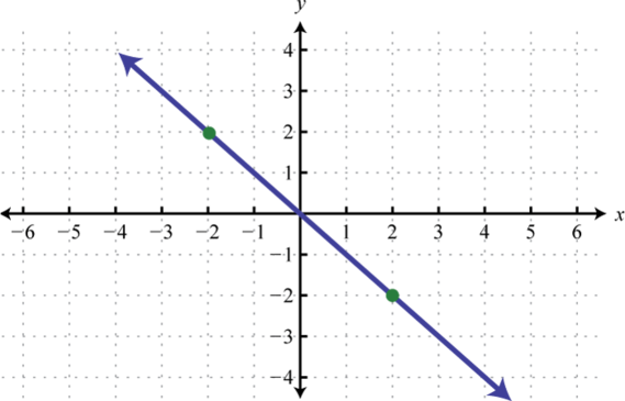
Example \(\PageIndex{4}\):
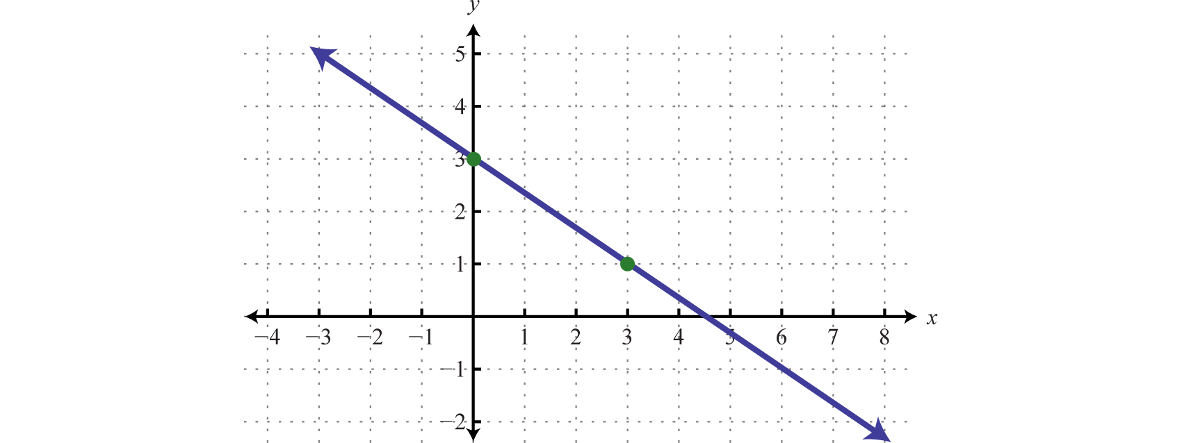
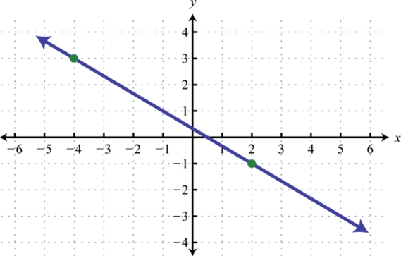
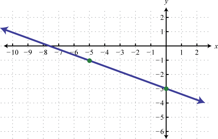
Determine a linear function that defines the given graph and find the \(x\)-intercept.
Solution
We begin by reading the slope from the graph. In this case, two points are given and we can see that,
\(m = \frac { r i s e } { r u n } = \frac { - 2 } { 3 }\)
In addition, the \(y\)-intercept is \((0, 3)\) and thus \(b=3\). We can substitute into the equation for any linear function.
\(\begin{array} { c } { g ( x ) = m x + b } \\ \quad\quad\quad\color{Cerulean}{\downarrow\quad\quad\downarrow} \\ { g ( x ) = - \frac { 2 } { 3 } x + 3 } \end{array}\)
To find the \(x\)-intercept, we set \(g(x)=0\) and solve for \(x\).
\(\begin{aligned} g ( x ) & = - \frac { 2 } { 3 } x + 3 \\ 0 & = - \frac { 2 } { 3 } x + 3 \\ \frac { 2 } { 3 } x & = 3 \\ \left( \color{Cerulean}{\frac { 3 } { 2 }} \right) \frac { 2 } { 3 } x & = \left( \color{Cerulean}{\frac { 3 } { 2 }} \right) 3 \\ x & = \frac { 9 } { 2 } = 4 \frac { 1 } { 2 } \end{aligned}\)
Answer:
\(g(x)=−\frac{2}{3}x+3\); \(x\)-intercept: \((\frac{9}{2},0)\)
Next, consider horizontal and vertical lines. Use the vertical line test to see that any horizontal line represents a function, and that a vertical line does not.
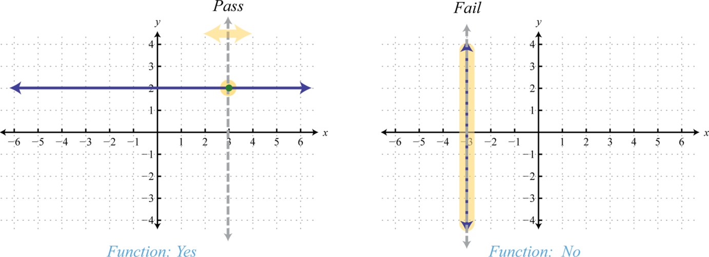
Given any horizontal line, the vertical line test shows that every \(x\)-value in the domain corresponds to exactly one \(y\)-value in the range; it is a function. A vertical line, on the other hand, fails the vertical line test; it is not a function. A vertical line represents a set of ordered pairs where all of the elements in the domain are the same. This violates the requirement that functions must associate exactly one element in the range to each element in the domain. We summarize as follows:
| Horizontal Line | Vertical Line | |
|---|---|---|
| Equation: | \(y=2\) | \(x=-3\) |
| \(x\)-intercept: | None | \((-3,0)\) |
| \(y\)-intercept: | \((0,2)\) | None |
| Domain: | \(( - \infty , \infty )\) | \(\{ - 3 \}\) |
| Range: | \(\{ 2 \}\) | \(( - \infty , \infty )\) |
| Function: | Yes | No |
A horizontal line is often called a constant function. Given any real number \(c\),
\(f ( x ) = c\:\:\:\color{Cerulean}{Constant\: Function}\)
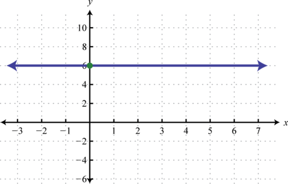
Example \(\PageIndex{5}\):
Graph the constant function \(g(x)=−2\) and state the domain and range.
Solution
Here we are given a constant function that is equivalent to \(y=−2\). This defines a horizontal line through \((0,−2)\).
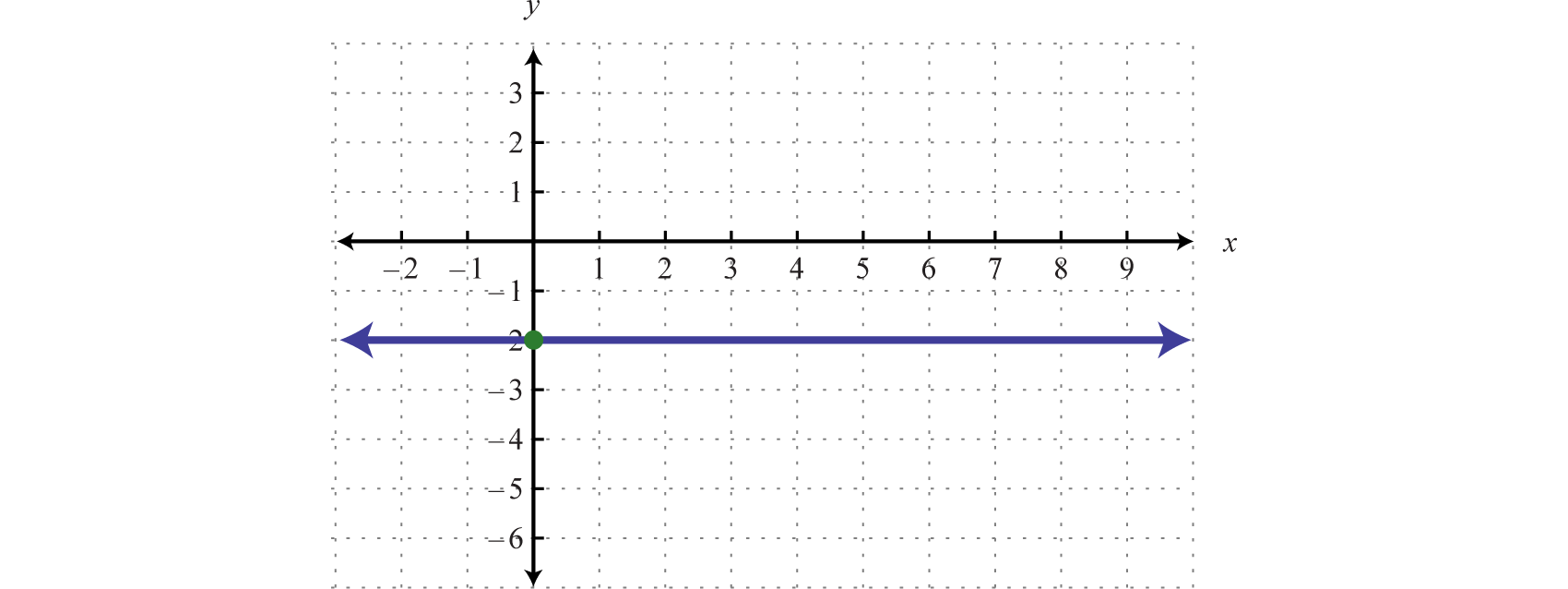
Answer:
Domain: \(ℝ\); range: \(\{−2\}\)
Exercise \(\PageIndex{1}\)
Graph \(f(x)=3x−2\) and label the \(x\)-intercept.
- Answer
-
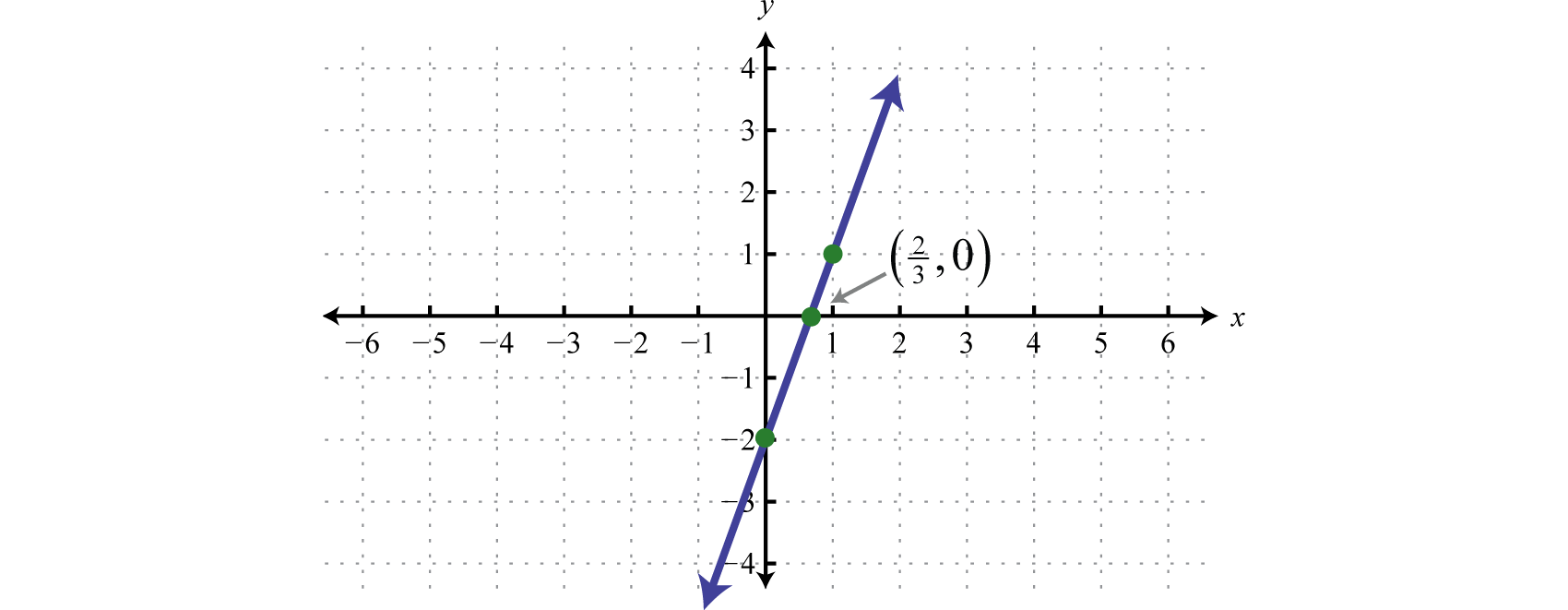
Figure \(\PageIndex{15}\) www.youtube.com/v/iyePPmPaMlA
Linear Equations and Inequalities: A Graphical Interpretation
We can use the ideas in this section to develop a geometric understanding of what it means to solve equations of the form \(f (x) = g (x)\), where \(f\) and \(g\) are linear functions. Using algebra, we can solve the linear equation \(\frac{1}{2} x + 1 = 3\) as follows:
\(\begin{aligned} \frac { 1 } { 2 } x + 1 & = 3 \\ \frac { 1 } { 2 } x & = 2 \\ (\color{Cerulean}{ 2 }\color{Black}{)} \frac { 1 } { 2 } x & = ( \color{Cerulean}{2}\color{Black}{)} 2 \\ x & = 4 \end{aligned}\)
The solution to this equation is \(x = 4\). Geometrically, this is the \(x\)-value of the intersection of the two graphs \(f (x) = \frac{1}{2} x + 1\) and \(g (x) = 3\). The idea is to graph the linear functions on either side of the equation and determine where the graphs coincide.
Example \(\PageIndex{6}\):
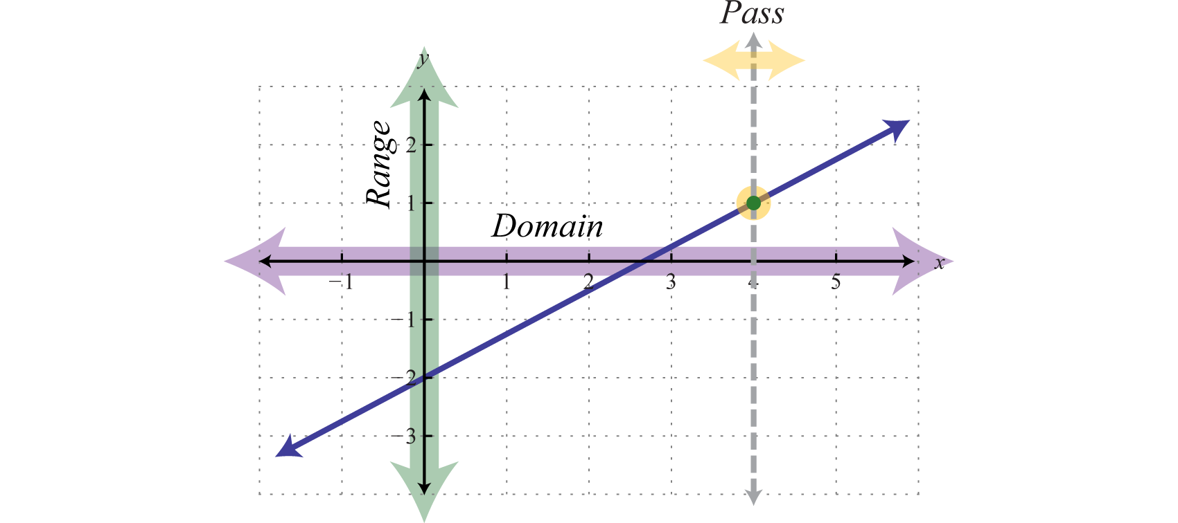
Graph \(f(x)=\frac{1}{2}x+1\) and \(g(x)=3\) on the same set of axes and determine where \(f(x)=g(x)\).
Solution
Here \(f\) is a linear function with slope \(\frac{1}{2}\) and \(y\)-intercept \((0,1)\). The function \(g\) is a constant function and represents a horizontal line. Graph both of these functions on the same set of axes.
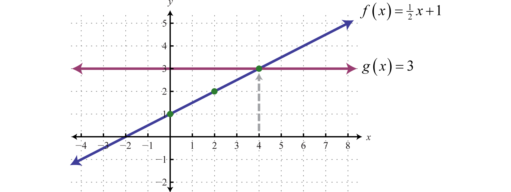
From the graph we can see that \(f(x)=g(x)\) where \(x=4\). In other words, \(\frac{1}{2}x+1=3\) where \(x=4\).
Answer:
\(x = 4\)
We can extend the geometric interpretation a bit further to solve inequalities. For example, we can solve the linear inequality \(\frac{1}{2} x + 1 ≥ 3\), using algebra, as follows:
\(\begin{array} { c } { \frac { 1 } { 2 } x + 1 \geq 3 } \\ { \quad \frac { 1 } { 2 } x \geq 2 } \\ ({ \color{Cerulean}{ 2}\color{Black}{)} \frac { 1 } { 2 } x \geq ( \color{Cerulean}{2}\color{Black}{ )} 2 } \\ { x \geq 4 } \end{array}\)
The solution set consists of all real numbers greater than or equal to \(4\). Geometrically, these are the \(x\)-values for which the graph \(f (x) = 1 2 x + 1\) lies above the graph of \(g (x) = 3\).
Example \(\PageIndex{7}\):
Graph \(f(x)=\frac{1}{2}x+1\) and \(g(x)=3\) on the same set of axes and determine where \(f(x)≥g(x)\).
Solution
On the graph we can see this shaded.
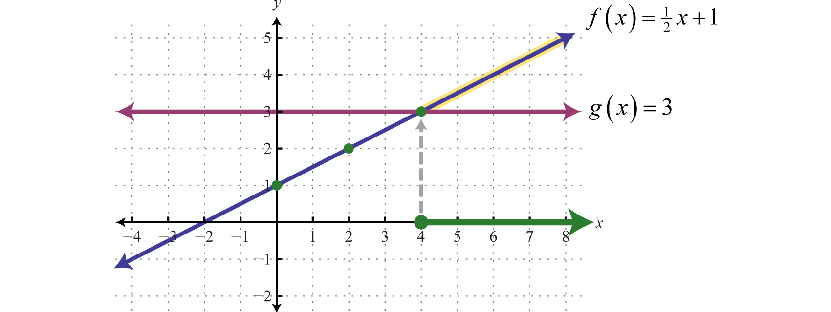
From the graph we can see that \(f(x)≥g(x)\) or \(\frac{1}{2}x+1≥3\) where \(x≥4\).
Answer:
The \(x\)-values that solve the inequality, in interval notation, are \([4,∞)\).
Key Takeaways
- We can graph lines by plotting points. Choose a few values for \(x\), find the corresponding \(y\)-values, and then plot the resulting ordered pair solutions. Draw a line through the points with a straightedge to complete the graph.
- Given any two points on a line, we can calculate the slope algebraically using the slope formula, \(m = \frac{rise}{run} = \frac{y_{2}−y_{1}}{x_{2}−x_{1}} = \frac{Δy}{Δx}\).
- Use slope-intercept form \(y = mx + b\) to quickly sketch the graph of a line. From the \(y\)-intercept \((0, b)\), mark off the slope to determine a second point. Since two points determine a line, draw a line through these two points with a straightedge to complete the graph.
- Linear functions have the form \(f (x) = mx + b\), where the slope \(m\) and \(b\) are real numbers. To find the \(x\)-intercept, if one exists, set \(f (x) = 0\: \)and solve for \(x\).
- Since \(y = f (x)\) we can use \(y\) and \(f (x)\) interchangeably. Any point on the graph of a function can be expressed using function notation \((x, f (x))\).
Exercise \(\PageIndex{2}\)
Find five ordered pair solutions and graph.
- \(y = 3x − 6\)
- \(y = 2x − 4\)
- \(y = −5x + 15\)
- \(y = −3x + 18\)
- \(y = \frac{1}{2} x + 8\)
- \(y = \frac{2}{3} x + 2\)
- \(y = −\frac{3}{5} x + 1\)
- \(y = −\frac{3}{2} x + 4\)
- \(y = \frac{1}{4} x\)
- \(y = −\frac{2}{5} x\)
- \(y = 10\)
- \(x = −1\)
- \(6x + 3y = 18\)
- \(8x − 2y = 16\)
- \(−2x + 4y = 8\)
- \(−x + 3y = 18\)
- \(\frac{1}{2} x − \frac{1}{5} y = 1\)
- \(\frac{1}{6} x − \frac{2}{3} y = 2\)
- \(x + y = 0\)
- \(−x + y = 0\)
- Answer
-
1.
Figure \(\PageIndex{18}\) 3.
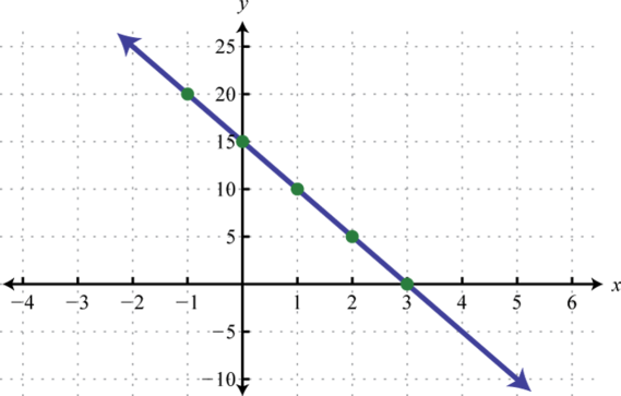
Figure \(\PageIndex{19}\) 5.
Figure \(\PageIndex{20}\) 7.
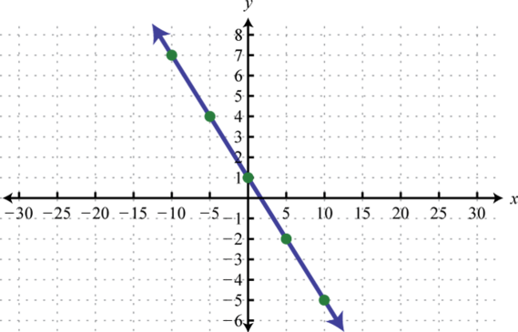
Figure \(\PageIndex{21}\) 9.
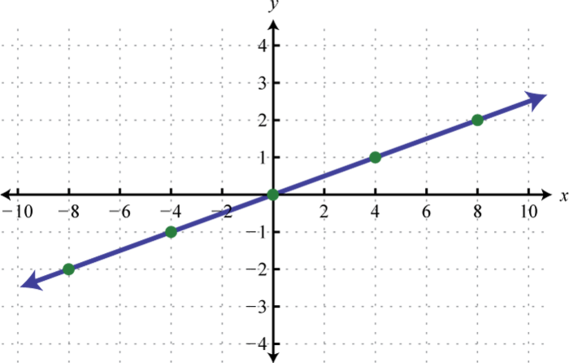
Figure \(\PageIndex{22}\) 11.
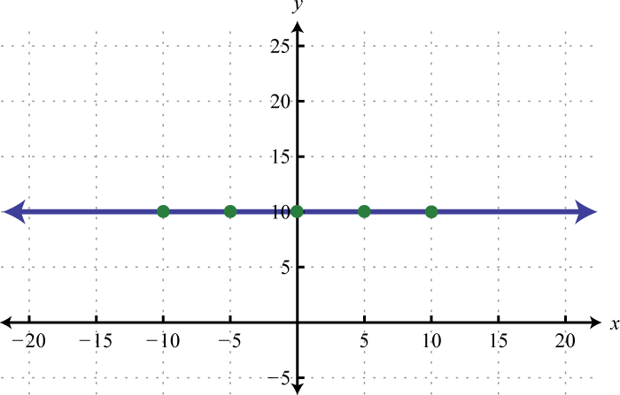
Figure \(\PageIndex{23}\) 13.
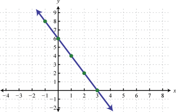
Figure \(\PageIndex{24}\) 15.
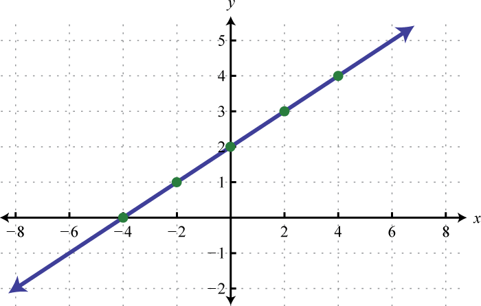
Figure \(\PageIndex{25}\) 17.
Figure \(\PageIndex{26}\) 19.
Figure \(\PageIndex{27}\)
Exercise \(\PageIndex{3}\)
Find the slope of the line passing through the given points.
- \((-2, -4)\) and \((1, -1)\)
- \((-3,0)\) and \((3, -4)\)
- \((-\frac{5}{2}, \frac{1}{4})\) and \((-\frac{1}{2}, \frac{5}{4})\)
- \((-4, -3)\) and \((-2, -3)\)
- \((9, -5)\) and \((9, -6)\)
- \((\frac{1}{2}, -1)\) and \((-1, -\frac{3}{2})\)
- Answer
-
1. \(1\)
3. \(\frac{1}{2}\)
5. Undefined
Exercise \(\PageIndex{4}\)
Find the \(y\)-value for which the slope of the line passing through given points has the given slope.
- \(m = \frac { 3 } { 2 } ; ( 6,10 ) , ( - 4 , y )\)
- \(m = - \frac { 1 } { 3 } ; ( - 6,4 ) , ( 9 , y )\)
- \(m = - 4 ; ( - 2,5 ) , ( - 1 , y )\)
- \(m = 3 ; ( 1 , - 2 ) , ( - 2 , y )\)
- \(m = \frac { 1 } { 5 } ; ( 1 , y ) , \left( 6 , \frac { 1 } { 5 } \right)\)
- \(m = - \frac { 3 } { 4 } ; ( - 1 , y ) , ( - 4,5 )\)
- Answer
-
1. \(y=-5\)
3. \(y=1\)
5. \(y=-\frac{4}{5}\)
Exercise \(\PageIndex{5}\)
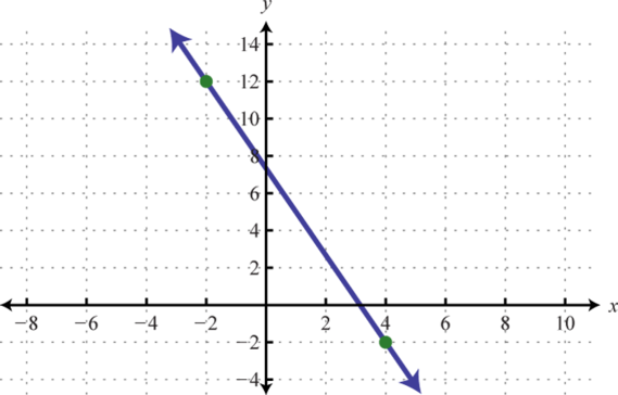
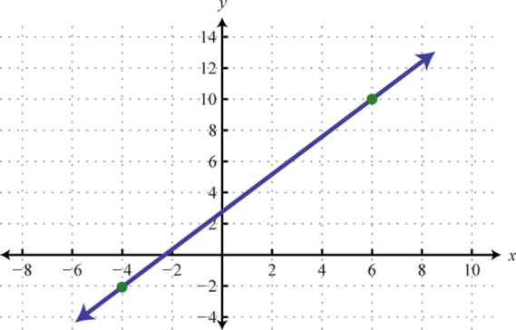
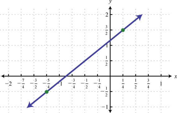
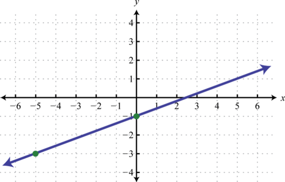
Given the graph, determine the slope.
1.
2.
3.
4.
5.
6.
7.
8.
- Answer
-
1. \(m = \frac { 1 } { 3 }\)
3. \(m = - \frac { 7 } { 3 }\)
5. \(m = \frac { 4 } { 3 }\)
7. \(m=0\)
Exercise \(\PageIndex{6}\)
Find the \(x\)- and \(y\)-intercepts and use them to graph the following functions.
- \(6x − 3y = 18\)
- \(8x − 2y = 8\)
- \(−x + 12y = 6\)
- \(−2x − 6y = 8\)
- \(x − 2y = 5\)
- \(−x + 3y = 1\)
- \(2x + 3y = 2\)
- \(5x − 4y = 2\)
- \(9x − 4y = 30\)
- \(−8x + 3y = 28\)
- \(\frac{1}{3} x + \frac{1}{2} y = −3\)
- \(\frac{1}{4} x − \frac{1}{3} y = 3\)
- \(\frac{7}{9} x − \frac{2}{3} y = \frac{14}{3}\)
- \(\frac{1}{8} x − \frac{1}{6} y = −\frac{3}{2}\)
- \(−\frac{1}{6} x + \frac{2}{9} y = \frac{4}{3}\)
- \(\frac{2}{15} x + \frac{1}{6} y = \frac{4}{3}\)
- \(y = −\frac{1}{4} x + \frac{1}{2}\)
- \(y = \frac{3}{8} x −\frac{3}{2}\)
- \(y = \frac{2}{3} x + \frac{1}{2}\)
- \(y = \frac{4}{5} x + 1\)
- Answer
-
1.
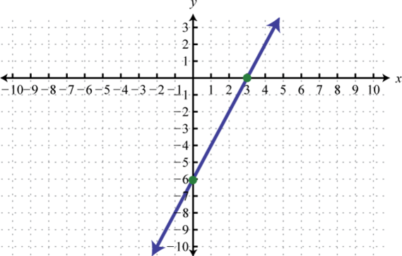
Figure \(\PageIndex{36}\) 3.
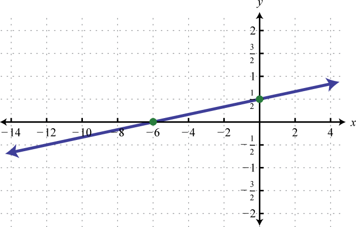
Figure \(\PageIndex{37}\) 5.
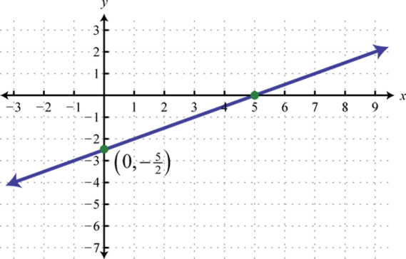
Figure \(\PageIndex{38}\) 7.
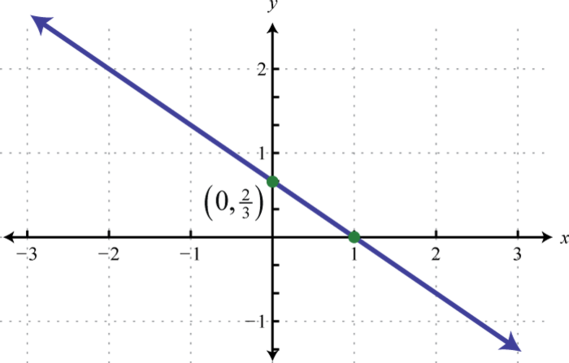
Figure \(\PageIndex{39}\) 9.
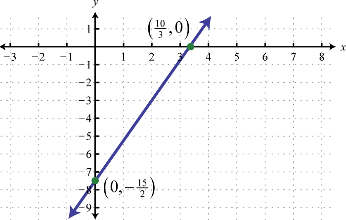
Figure \(\PageIndex{40}\) 11.
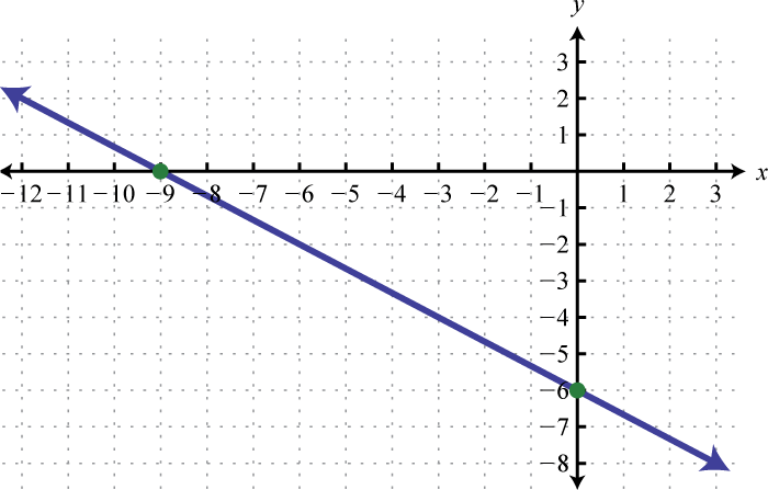
Figure \(\PageIndex{41}\) 13.
Figure \(\PageIndex{42}\) 15.
Figure \(\PageIndex{43}\) 17.
Figure \(\PageIndex{44}\) 19.
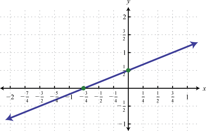
Figure \(\PageIndex{45}\)
Exercise \(\PageIndex{7}\)
Graph the linear function and label the \(x\)-intercept.
- \(f (x) = −5x + 15\)
- \(f (x) = −2x + 6\)
- \(f (x) = −x − 2\)
- \(f (x) = x + 3\)
- \(f (x) = \frac{1}{3} x + 2\)
- \(f (x) = \frac{5}{2} x + 10\)
- \(f (x) = \frac{5}{3} x + 2\)
- \(f (x) = \frac{2}{5} x − 3\)
- \(f (x) = −\frac{5}{6} x + 2\)
- \(f (x) = −\frac{4}{3} x + 3\)
- \(f (x) = 2x\)
- \(f (x) = 3\)
- Answer
-
1.
Figure \(\PageIndex{46}\) 3.
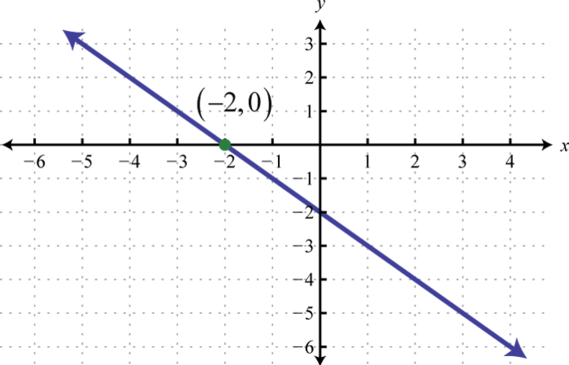
Figure \(\PageIndex{47}\) 5.
Figure \(\PageIndex{48}\) 7.
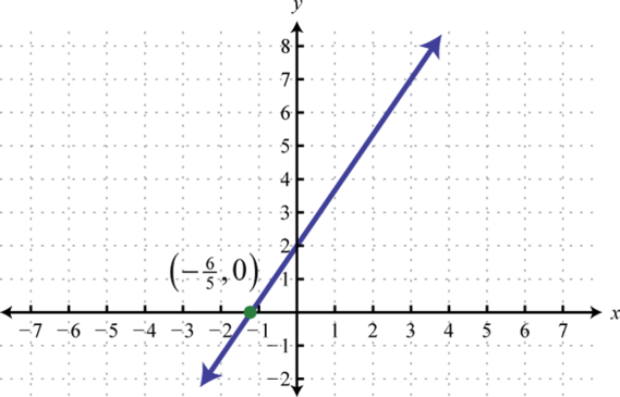
Figure \(\PageIndex{49}\) 9.
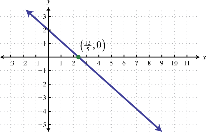
Figure \(\PageIndex{50}\) 11.
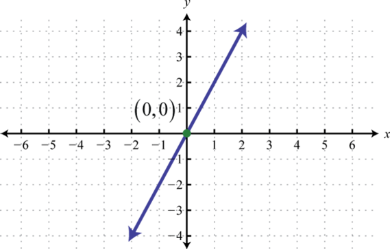
Figure \(\PageIndex{51}\)
Exercise \(\PageIndex{8}\)
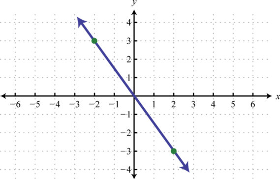
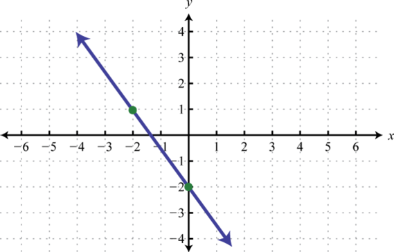
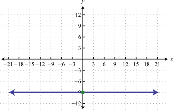
Determine the linear function that defines the given graph and find the \(x\)-intercept.
1.
2.
3.
4.
5.
6.
7.
8.
- Answer
-
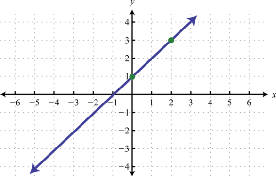
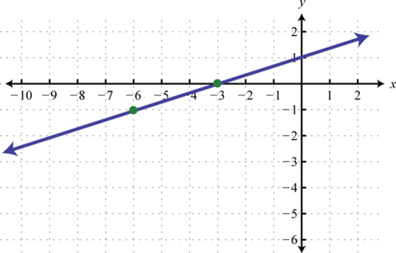
1. \(f (x) = x + 1; (−1, 0)\)
3. \(f (x) = −\frac{3}{2} x; (0, 0)\)
5. \(f (x) = −9;\) none
7. \(f (x) = \frac{1}{3} x + 1; (−3, 0)\)
Exercise \(\PageIndex{9}\)
Graph the functions \(f\) and \(g\) on the same set of axes and determine where \(f(x)=g(x)\). Verify your answer algebraically.
- \(f (x) = \frac{1}{2} x − 3, g (x) = 1\)
- \(f (x) = \frac{1}{3} x + 2, g (x) = −1\)
- \(f (x) = 3x − 2 , g (x) = −5\)
- \(f (x) = x + 2, g (x) = −3\)
- \(f (x) = −\frac{2}{3} x + 4, g (x) = 2\)
- \(f (x) = −\frac{5}{2} x + 6, g (x) = 1\)
- \(f (x) = 3x − 2 , g (x) = −2x + 3\)
- \(f (x) = −x + 6, g (x) = x + 2\)
- \(f (x) = −\frac{1}{3} x, g (x) = −\frac{2}{3} x + 1\)
- \(f (x) = \frac{2}{3} x − 1, g (x) = −\frac{4}{3} x − 3\)
- Answer
-
1. \(x = 8\)
3. \(x = −1\)
5. \(x = 3\)
7. \(x = 1\)
9. \(x = 3\)
Exercise \(\PageIndex{10}\)
Graph the functions \(f\) and \(g\) on the same set of axes and determine where \(f(x)\geq g(x)\). Verify your answer algebraically.
- \(f (x) = 3x + 7 , g (x) = 1\)
- \(f (x) = 5x − 3 , g (x) = 2\)
- \(f (x) = \frac{2}{3} x − 3, g (x) = −3\)
- \(f (x) = \frac{3}{4} x + 2, g (x) = −1\)
- \(f (x) = −x + 1, g (x) = −3\)
- \(f (x) = −4x + 4 , g (x) = 8\)
- \(f (x) = x − 2, g (x) = −x + 4\)
- \(f (x) = 4x − 5 , g (x) = x + 1\)
- Answer
-
1. \([ - 2 , \infty )\)
3. \([ 0 , \infty )\)
5. \(( - \infty , 4 ]\)
7. \([ 3 , \infty )\)
Exercise \(\PageIndex{11}\)
Graph the functions \(f\) and \(g\) on the same set of axes and determine where \(f(x)<g(x)\). Verify your answer algebraically.
- \(f (x) = x + 5, g (x) = −1\)
- \(f (x) = 3x − 3 , g (x) = 6\)
- \(f (x) = −\frac{4}{5} x, g (x) = −8\)
- \(f (x) = −\frac{3}{2} x + 6, g (x) = −3\)
- \(f (x) = \frac{1}{4} x + 1, g (x) = 0\)
- \(f (x) = \frac{3}{5} x − 6, g (x) = 0\)
- \(f (x) = \frac{1}{3} x + 2, g (x) = − \frac{1}{3} x\)
- \(f (x) = \frac{3}{2} x + 3, g (x) = −\frac{3}{2} x − 3\)
- Answer
-
1. \(( - \infty , - 6 )\)
3. \(( 10 , \infty )\)
5. \(( - \infty , - 4 )\)
7. \(( - \infty , - 3 )\)
Exercise \(\PageIndex{12}\)
- Do all linear functions have \(y\)-intercepts? Do all linear functions have \(x\)-intercepts? Explain.
- Can a function have more than one \(y\)-intercept? Explain.
- How does the vertical line test show that a vertical line is not a function?
- Answer
-
1. Answer may vary
3. Answer may vary
Footnotes
18The variable that determines the values of other variables. Usually we think of the \(x\)-value of an ordered pair \((x, y)\) as the independent variable.
19The variable whose value is determined by the value of the independent variable. Usually we think of the \(y\)-value of an ordered pair \((x, y)\) as the dependent variable.
20A way of determining a graph using a finite number of representative ordered pair solutions.
21The incline of a line measured as the ratio of the vertical change to the horizontal change, often referred to as “rise over run.”
22The vertical change between any two points on a line.
23The horizontal change between any two points on a line.
24The slope of the line through the points \((x1, y1)\) and \((x2, y2)\) is given by the formula \(m = \frac{y2−y1}{x2−x1}\).
25Any nonvertical line can be written in the standard form \(ax + by = c\).
26Any nonvertical line can be written in the form \(y = mx + b\), where \(m\) is the slope and \((0, b)\) is the \(y\)-intercept.
27The point (or points) where a graph intersects the y-axis, expressed as an ordered pair \((0, y)\).
28Any function that can be written in the form f (x) = mx + b
29The point (or points) where a graph intersects the x-axis, expressed as an ordered pair (x, 0).