2.3: Modeling Linear Functions
- Page ID
- 6235
\( \newcommand{\vecs}[1]{\overset { \scriptstyle \rightharpoonup} {\mathbf{#1}} } \)
\( \newcommand{\vecd}[1]{\overset{-\!-\!\rightharpoonup}{\vphantom{a}\smash {#1}}} \)
\( \newcommand{\dsum}{\displaystyle\sum\limits} \)
\( \newcommand{\dint}{\displaystyle\int\limits} \)
\( \newcommand{\dlim}{\displaystyle\lim\limits} \)
\( \newcommand{\id}{\mathrm{id}}\) \( \newcommand{\Span}{\mathrm{span}}\)
( \newcommand{\kernel}{\mathrm{null}\,}\) \( \newcommand{\range}{\mathrm{range}\,}\)
\( \newcommand{\RealPart}{\mathrm{Re}}\) \( \newcommand{\ImaginaryPart}{\mathrm{Im}}\)
\( \newcommand{\Argument}{\mathrm{Arg}}\) \( \newcommand{\norm}[1]{\| #1 \|}\)
\( \newcommand{\inner}[2]{\langle #1, #2 \rangle}\)
\( \newcommand{\Span}{\mathrm{span}}\)
\( \newcommand{\id}{\mathrm{id}}\)
\( \newcommand{\Span}{\mathrm{span}}\)
\( \newcommand{\kernel}{\mathrm{null}\,}\)
\( \newcommand{\range}{\mathrm{range}\,}\)
\( \newcommand{\RealPart}{\mathrm{Re}}\)
\( \newcommand{\ImaginaryPart}{\mathrm{Im}}\)
\( \newcommand{\Argument}{\mathrm{Arg}}\)
\( \newcommand{\norm}[1]{\| #1 \|}\)
\( \newcommand{\inner}[2]{\langle #1, #2 \rangle}\)
\( \newcommand{\Span}{\mathrm{span}}\) \( \newcommand{\AA}{\unicode[.8,0]{x212B}}\)
\( \newcommand{\vectorA}[1]{\vec{#1}} % arrow\)
\( \newcommand{\vectorAt}[1]{\vec{\text{#1}}} % arrow\)
\( \newcommand{\vectorB}[1]{\overset { \scriptstyle \rightharpoonup} {\mathbf{#1}} } \)
\( \newcommand{\vectorC}[1]{\textbf{#1}} \)
\( \newcommand{\vectorD}[1]{\overrightarrow{#1}} \)
\( \newcommand{\vectorDt}[1]{\overrightarrow{\text{#1}}} \)
\( \newcommand{\vectE}[1]{\overset{-\!-\!\rightharpoonup}{\vphantom{a}\smash{\mathbf {#1}}}} \)
\( \newcommand{\vecs}[1]{\overset { \scriptstyle \rightharpoonup} {\mathbf{#1}} } \)
\(\newcommand{\longvect}{\overrightarrow}\)
\( \newcommand{\vecd}[1]{\overset{-\!-\!\rightharpoonup}{\vphantom{a}\smash {#1}}} \)
\(\newcommand{\avec}{\mathbf a}\) \(\newcommand{\bvec}{\mathbf b}\) \(\newcommand{\cvec}{\mathbf c}\) \(\newcommand{\dvec}{\mathbf d}\) \(\newcommand{\dtil}{\widetilde{\mathbf d}}\) \(\newcommand{\evec}{\mathbf e}\) \(\newcommand{\fvec}{\mathbf f}\) \(\newcommand{\nvec}{\mathbf n}\) \(\newcommand{\pvec}{\mathbf p}\) \(\newcommand{\qvec}{\mathbf q}\) \(\newcommand{\svec}{\mathbf s}\) \(\newcommand{\tvec}{\mathbf t}\) \(\newcommand{\uvec}{\mathbf u}\) \(\newcommand{\vvec}{\mathbf v}\) \(\newcommand{\wvec}{\mathbf w}\) \(\newcommand{\xvec}{\mathbf x}\) \(\newcommand{\yvec}{\mathbf y}\) \(\newcommand{\zvec}{\mathbf z}\) \(\newcommand{\rvec}{\mathbf r}\) \(\newcommand{\mvec}{\mathbf m}\) \(\newcommand{\zerovec}{\mathbf 0}\) \(\newcommand{\onevec}{\mathbf 1}\) \(\newcommand{\real}{\mathbb R}\) \(\newcommand{\twovec}[2]{\left[\begin{array}{r}#1 \\ #2 \end{array}\right]}\) \(\newcommand{\ctwovec}[2]{\left[\begin{array}{c}#1 \\ #2 \end{array}\right]}\) \(\newcommand{\threevec}[3]{\left[\begin{array}{r}#1 \\ #2 \\ #3 \end{array}\right]}\) \(\newcommand{\cthreevec}[3]{\left[\begin{array}{c}#1 \\ #2 \\ #3 \end{array}\right]}\) \(\newcommand{\fourvec}[4]{\left[\begin{array}{r}#1 \\ #2 \\ #3 \\ #4 \end{array}\right]}\) \(\newcommand{\cfourvec}[4]{\left[\begin{array}{c}#1 \\ #2 \\ #3 \\ #4 \end{array}\right]}\) \(\newcommand{\fivevec}[5]{\left[\begin{array}{r}#1 \\ #2 \\ #3 \\ #4 \\ #5 \\ \end{array}\right]}\) \(\newcommand{\cfivevec}[5]{\left[\begin{array}{c}#1 \\ #2 \\ #3 \\ #4 \\ #5 \\ \end{array}\right]}\) \(\newcommand{\mattwo}[4]{\left[\begin{array}{rr}#1 \amp #2 \\ #3 \amp #4 \\ \end{array}\right]}\) \(\newcommand{\laspan}[1]{\text{Span}\{#1\}}\) \(\newcommand{\bcal}{\cal B}\) \(\newcommand{\ccal}{\cal C}\) \(\newcommand{\scal}{\cal S}\) \(\newcommand{\wcal}{\cal W}\) \(\newcommand{\ecal}{\cal E}\) \(\newcommand{\coords}[2]{\left\{#1\right\}_{#2}}\) \(\newcommand{\gray}[1]{\color{gray}{#1}}\) \(\newcommand{\lgray}[1]{\color{lightgray}{#1}}\) \(\newcommand{\rank}{\operatorname{rank}}\) \(\newcommand{\row}{\text{Row}}\) \(\newcommand{\col}{\text{Col}}\) \(\renewcommand{\row}{\text{Row}}\) \(\newcommand{\nul}{\text{Nul}}\) \(\newcommand{\var}{\text{Var}}\) \(\newcommand{\corr}{\text{corr}}\) \(\newcommand{\len}[1]{\left|#1\right|}\) \(\newcommand{\bbar}{\overline{\bvec}}\) \(\newcommand{\bhat}{\widehat{\bvec}}\) \(\newcommand{\bperp}{\bvec^\perp}\) \(\newcommand{\xhat}{\widehat{\xvec}}\) \(\newcommand{\vhat}{\widehat{\vvec}}\) \(\newcommand{\uhat}{\widehat{\uvec}}\) \(\newcommand{\what}{\widehat{\wvec}}\) \(\newcommand{\Sighat}{\widehat{\Sigma}}\) \(\newcommand{\lt}{<}\) \(\newcommand{\gt}{>}\) \(\newcommand{\amp}{&}\) \(\definecolor{fillinmathshade}{gray}{0.9}\)Learning Objectives
- Determine the equation of a line given two points.
- Determine the equation of a line given the slope and \(y\)-intercept.
- Find linear functions that model common applications.
Equations of Lines
Given the algebraic equation of a line, we can graph it in a number of ways. In this section, we will be given a geometric description of a line and find the algebraic equation. Finding the equation of a line can be accomplished in a number of ways. The following example makes use of slope-intercept form, \(y = mx + b\), or using function notation, \(f (x) = mx + b\). If we can determine the slope, \(m\), and the \(y\)-intercept, \((0, b)\), we can then construct the equation.
Example \(\PageIndex{1}\):
Find the equation of the line passing through \((−3, 6)\) and \((5, −4)\).
Solution
We begin by finding the slope. Given two points, we can find the slope using the slope formula.
\(\begin{array} { l l } { \left( x _ { 1 } , y _ { 1 } \right) } & { \left( x _ { 2 } , y _ { 2 } \right) } \\ { ( - 3,6 ) } & { ( 5 , - 4 ) } \end{array}\)
\(\begin{aligned} m & = \frac { y _ { 2 } - y _ { 1 } } { x _ { 2 } - x _ { 1 } } \\ & = \frac { - 4 - ( 6 ) } { 5 - ( - 3 ) } \\ & = \frac { - 4 - 6 } { 5 + 3 } \\ & = \frac { - 10 } { 8 } \\ & = - \frac { 5 } { 4 } \end{aligned}\)
Here \(m = −\frac{5}{4}\) and we have
\(\begin{array} { l } { f ( x ) = m x + b } \\ { f ( x ) = - \frac { 5 } { 4 } x + b } \end{array}\)
To find \(b\), substitute either one of the given points through which the line passes. Here we will use \((−3, 6)\), but \((5, −4)\) would work just as well:
\(\begin{aligned} f ( x ) & = - \frac { 5 } { 4 } x + b \quad\quad\color{Cerulean} {Use (x, f(x))=(-3,6)} \\ \color{OliveGreen}{6} & \color{Black}{=} - \frac { 5 } { 4 } ( \color{OliveGreen}{- 3}\color{Black}{ )} + b \\ 6 & = \frac { 15 } { 4 } + b \\ \frac { 6 \cdot \color{Cerulean}{4} } { \color{Black}{1} \cdot \color{Cerulean}{4} } - \frac { 15 } { 4 } & = b \\ \frac { 24-15 } { 4 } - 15 \\ \frac { 9 } { 4 } & = b \end{aligned}\)
Therefore, the equation of the line passing through the two given points is:
\(\begin{array} { l } { f ( x ) = m x \:\:+\:\: b } \\ \quad\quad\quad\quad\color{Cerulean}{\downarrow\quad\:\:\:\:\:\downarrow} \\ { f ( x ) = - \frac { 5 } { 4 } x + \frac { 9 } { 4 } } \end{array}\)
Answer
\[f ( x ) = - \frac { 5 } { 4 } x + \frac { 9 } { 4 }\]
Next, we outline an alternative method for finding equations of lines. Begin by applying the slope formula with a given point \((x_{1} , y_{1})\) and a variable point \((x, y)\).
\(\begin{aligned} m & = \frac { y - y _ { 1 } } { x - x _ { 1 } } \\ \frac { m } { 1 } & = \frac { y - y _ { 1 } } { x - x _ { 1 } } \quad\quad\color{Cerulean}{Cross \:multiply}\\ m \left( x - x _ { 1 } \right) & = y - y _ { 1 } \quad\quad\color{Cerulean}{Apply \:the \:symmetric\: property}\\ \left( y - y _ { 1 } \right) & = m \left( x - x _ { 1 } \right) \end{aligned}\)
Therefore, the equation of a nonvertical line can be written in point-slope form30:
\(y - y _ { 1 } = m \left( x - x _ { 1 } \right) \quad\color{Cerulean}{Point-slope\: form.}\)
Point-slope form is particularly useful for finding the equation of a line given the slope and any ordered pair solution. After finding the slope, \(−\frac{5}{4}\) in the previous example, we could use this form to find the equation.
\(\begin{array} { l } { \color{Cerulean} { Point \quad\quad Slope } } \\ { \left( x _ { 1 } , y _ { 1 } \right) } \\ { ( - 3,6 ) \quad m = - \frac { 5 } { 4 } } \end{array}\)
Substitute as follows.
\(\begin{aligned} y - y _ { 1 } & = \color{Cerulean}{m} \color{Black}{\left( x - x _ { 1 } \right)} \\ y - ( \color{OliveGreen}{6}\color{Black}{ )} & = \color{Cerulean}{- \frac { 5 } { 4 } }\color{Black}{(} x - (\color{OliveGreen}{ - 3}\color{Black}{ )} ) \quad \color {Cerulean} { Solve\:for\: y } \\ y - 6 & = - \frac { 5 } { 4 } ( x + 3 ) \quad\quad\color{Cerulean} { Distribute } \\ y - 6 & = - \frac { 5 } { 4 } x - \frac { 15 } { 4 } \\ y & = - \frac { 5 } { 4 } x - \frac { 15 } { 4 } +6 \\ y & = - \frac { 5 } { 4 } x + \frac { 9 } { 4 } \end{aligned}\)
Notice that we obtain the same linear function \(f ( x ) = - \frac { 5 } { 4 } x + \frac { 9 } { 4 }\).
Sometimes a variable is not expressed explicitly in terms of another; however, it is still assumed that one variable is dependent on the other. For example, the equation \(2x + 3y = 6\) implicitly represents the function \(f (x) = −\frac{2}{3}x + 2\).You should become comfortable with working with functions in either form.
Example \(\PageIndex{2}\)
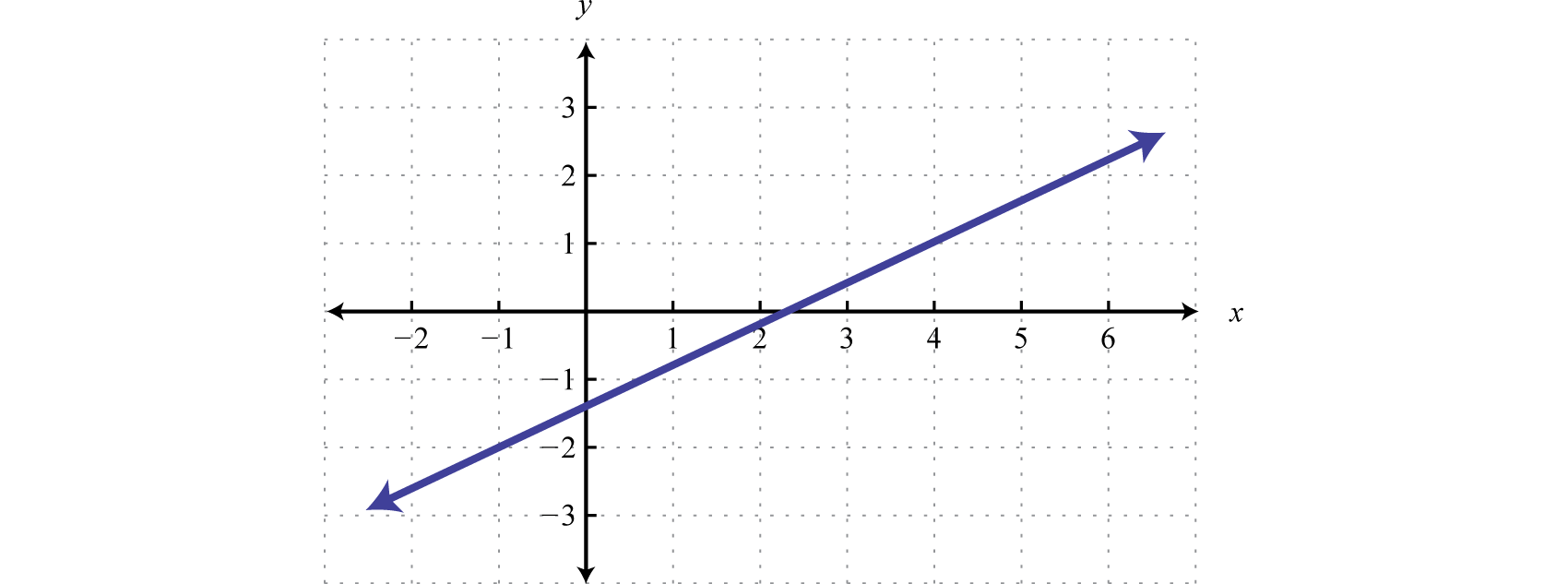
Find the equation of the following linear function:
Solution
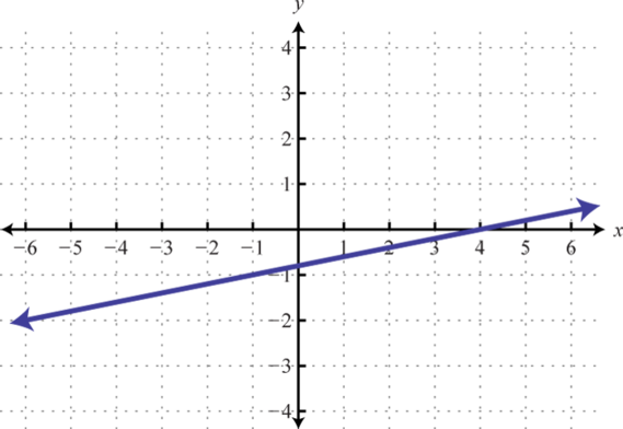
From the graph we can determine two points \((−1, −2)\) and \((4, 1)\). Use these points to read the slope from the graph. The rise is \(3\) units and the run is \(5\) units.
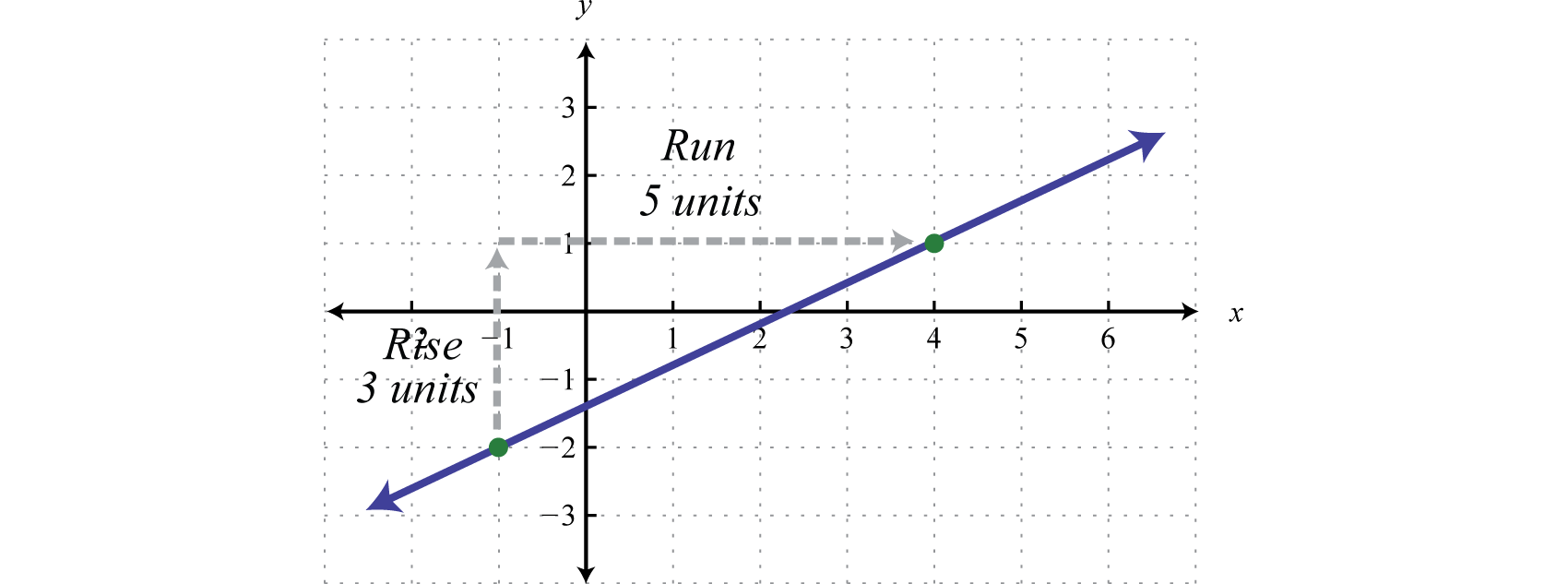
Therefore, we have the slope and a point. (It does not matter which of the given points we use, the result will be the same.)
\(\begin{array} { l } { \color{Cerulean} { Point } }\quad\quad\:\:\color{Cerulean}{Slope} \\ { ( - 1 , - 2 ) \quad m = \frac { 3 } { 5 } } \end{array}\)
Use point-slope form to determine the equation of the line.
\(\begin{aligned} y - y _ { 1 } & = \color{Cerulean}{m} \color{Black}{\left( x - x _ { 1 } \right)} \\ y - ( \color{OliveGreen}{- 2}\color{Black}{ )} & = \color{Cerulean}{\frac { 3 } { 5 }} \color{Black}{(} x - ( \color{OliveGreen}{- 1}\color{Black}{ )} ) \quad \color {Cerulean} { Solve\: for\: y. } \\ y + 2 & = \frac { 3 } { 5 } ( x + 1 ) \\ y + 2 & = \frac { 3 } { 5 } x + \frac { 3 } { 5 } \\ y & = \frac { 3 } { 5 } x + \frac { 3 } { 5 } - 2 \\ y & = \frac { 3 } { 5 } x - \frac { 7 } { 5 } \end{aligned}\)
Answer
\[f(x)=\frac{3}{5}x−\frac{7}{5}\]
Recall that parallel lines31 are lines in the same plane that never intersect. Two non-vertical lines in the same plane with slopes \(m_{1}\) and \(m_{2}\) are parallel if their slopes are the same, \(m_{1} = m_{2}\).
Example \(\PageIndex{3}\)
Find the equation of the line passing through \((3, −2)\) and parallel to \(x − 2y = −2\).
Solution
To find the slope of the given line, solve for \(y\).
\(\begin{aligned} x - 2 y & = - 2 \\ - 2 y & = - x - 2 \\ y & = \frac { - x - 2 } { - 2 } \\ y & = \frac { - x } { - 2 } - \frac { 2 } { - 2 } \\ y & = \frac { 1 } { 2 } x + 1 \end{aligned}\)
Here the given line has slope \(m = \frac{1}{2}\) and thus the slope of a parallel line \(m_{∥} = \frac{1}{2}\).The notation \(m_{∥}\) reads “\(m\) parallel.” Since we are given a point and we now have the slope, we will choose to use point-slope form of a line to determine the equation.
\(\begin{array} { l l } { \color{Cerulean}{ Point } } & { \color{Cerulean}{ Slope } } \\ { ( 3 , - 2 ) } & { m _ { \| } = \frac { 1 } { 2 } } \end{array}\)
\(\begin{aligned} y - y _ { 1 } & = m \left( x - x _ { 1 } \right) \color{Cerulean}{Point-Slope\: form}\\ y - ( - 2 ) & = \frac { 1 } { 2 } ( x - 3 ) \\ y + 2 & = \frac { 1 } { 2 } x - \frac { 3 } { 2 } \\ y + 2 \color{Cerulean}{- 2} & = \frac { 1 } { 2 } x - \frac { 3 } { 2 } \color{Cerulean}{- 2} \\ y & = \frac { 1 } { 2 } x - \frac { 7 } { 2 } \end{aligned}\)
Answer
\[f ( x ) = \frac { 1 } { 2 } x - \frac { 7 } { 2 }\]
It is important to have a geometric understanding of this question. We were asked to find the equation of a line parallel to another line passing through a certain point.
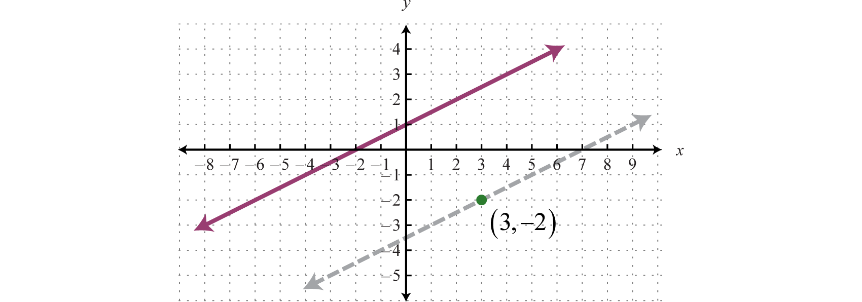
Through the point \((3, −2)\) we found a parallel line, \(y = \frac{1}{2} x − \frac{7}{2}\), shown as a dashed line. Notice that the slope is the same as the given line, \(y = \frac{1}{2} x + 1\), but the \(y\)-intercept is different.
Recall that perpendicular lines32 are lines in the same plane that intersect at right angles (\(90\) degrees). Two nonvertical lines, in the same plane with slopes \(m_{1}\) and \(m_{2}\), are perpendicular if the product of their slopes is \(−1\), \(m_{1} ⋅ m_{2} = −1\). We can solve for \(m_{1}\) and obtain \(m_{1} = −\frac{1}{m_{2}}\). In this form, we see that perpendicular lines have slopes that are negative reciprocals33, or opposite reciprocals34. In general, given real numbers a and b,
\(\text{If}\: m = \frac { a } { b } \text { then } m _ { \perp } = - \frac { b } { a }\)
The mathematical notation \(m_{⊥}\) reads “\(m\) perpendicular”. For example, the opposite reciprocal of \(m = −\frac{3}{5}\) is \(m⊥ = \frac{5}{3}\). We can verify that two slopes produce perpendicular lines if their product is \(−1\).
\(m \cdot m _ { \perp } = - \frac { 3 } { 5 } \cdot \frac { 5 } { 3 } = - \frac { 15 } { 15 } = - 1\color{Cerulean}{✓}\)
Example \(\PageIndex{4}\):
Find the equation of the line passing through \((−5, −2)\) and perpendicular to \(x + 4y = 4\).
Solution
To find the slope of the given line, solve for \(y\).
\(\begin{aligned} x + 4 y & = 4 \\ 4 y & = - x + 4 \\ y & = \frac { - x + 4 } { 4 } \\ y & = \frac { - x } { 4 } + \frac { 4 } { 4 } \\ y & = - \frac { 1 } { 4 } x + 1 \end{aligned}\)
The given line has slope \(m = −\frac{1}{4}\), and thus, \(m⊥ = +\frac{4}{1} = 4\). Substitute this slope and the given point into point-slope form.
\(\begin{array} { l l } { \color{Cerulean} { Point } } & { \color{Cerulean} { Slope } } \\ { ( - 5 , - 2 ) } & { m _ { \perp } = 4 } \end{array}\)
\(\begin{aligned} y - y _ { 1 } & = m \left( x - x _ { 1 } \right) \\ y - ( - 2 ) & = 4 ( x - ( - 5 ) ) \\ y + 2 & = 4 ( x + 5 ) \\ y + 5 & = 4 x + 20 \\ y & = 4 x + 18 \end{aligned}\)
Answer
\[f(x)=4x+18\]
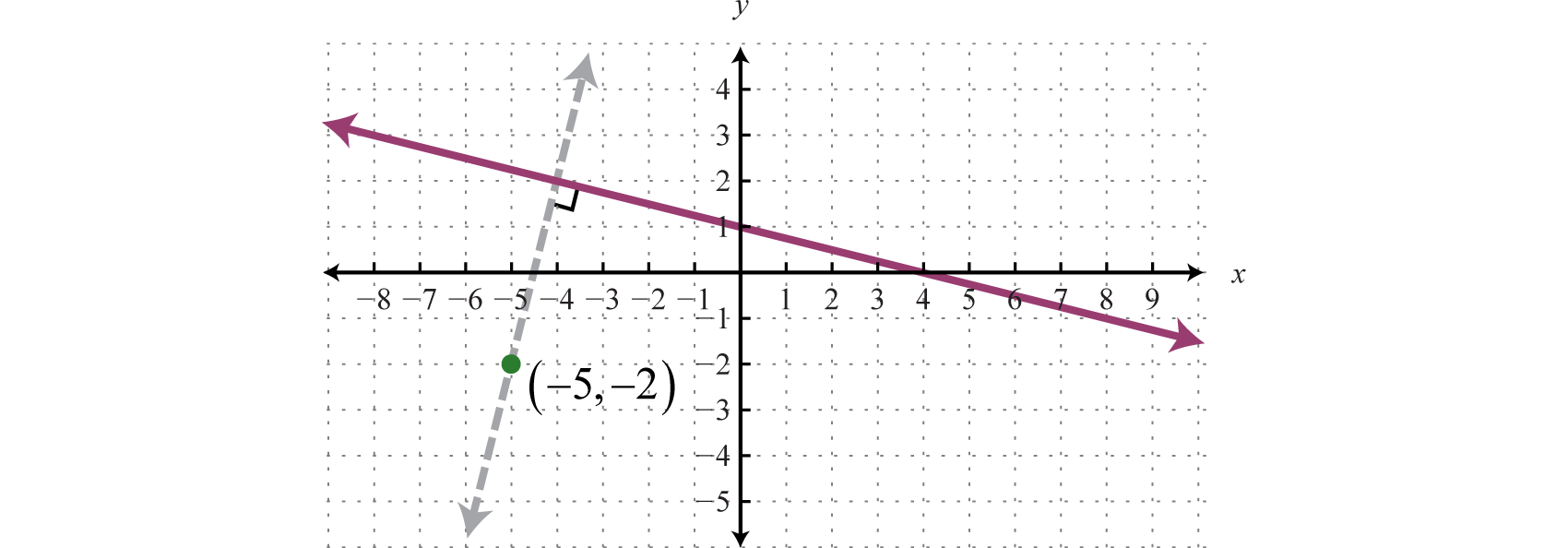
Geometrically, we see that the line \(y=4x+18\), shown as a dashed line in the graph, passes through \((-5, -2)\) and is perpendicular to the given line \(y=\frac{1}{4}x+1\).
Exercise \(\PageIndex{1}\)
Find the equation of the line passing through \((−5, −2)\) and perpendicular to \(\frac{1}{3} x − \frac{1}{2} y = −2\).
- Answer
-
\(y = - \frac { 3 } { 2 } x - \frac { 19 } { 2 }\)
www.youtube.com/v/nCnJw7jD2sk
Modeling Linear Applications
Data can be used to construct functions that model real-world applications. Once an equation that fits given data is determined, we can use the equation to make certain predictions; this is called mathematical modeling35.
Example \(\PageIndex{5}\):
The cost of a daily truck rental is \($48.00\), plus an additional \($0.45\) for every mile driven. Write a function that gives the cost of the daily truck rental and use it to determine the total cost of renting the truck for a day and driving it \(60\) miles.
Solution
The total cost of the truck rental depends on the number of miles driven. If we let \(x\) represent the number of miles driven, then \(0.45x\) represents the variable cost of renting the truck. Use this and the fixed cost, \($48.00\), to write a function that models the total cost,
\(C ( x ) = 0.45 x + 48\)
Use this function to calculate the cost of the rental when \(x = 60\) miles.
\(\begin{aligned} C ( 60 ) & = 0.45 ( 60 ) + 48 \\ & = 27 + 48 \\ & = 75 \end{aligned}\)
Answer:
The total cost of renting the truck for the day and driving it \(60\) miles would be \($75\).
We can use the model \(C (x) = 0.45x + 48\) to answer many more questions. For example, how many miles can be driven to keep the cost of the rental at most \($66\)? To answer this question, set up an inequality that expresses the cost less than or equal to \($66\).
\(\begin{aligned} C ( x ) & \leq \$ 66 \\ 0.45 x + 48 & \leq 66 \end{aligned}\)
Solve for \(x\) to determine the number of miles that can be driven.
\(\begin{aligned} 0.45 x + 48 & \leq 66 \\ 0.45 x & \leq 18 \\ x & \leq 40 \end{aligned}\)
To limit the rental cost to \($66\), the truck can be driven \(40\) miles or less.
Example \(\PageIndex{6}\):
A company purchased a new piece of equipment for \($12,000\). Four years later it was valued at \($9,000\) dollars. Use this data to construct a linear function that models the value of the piece of equipment over time.
Solution
The value of the item depends on the number of years after it was purchased. Therefore, the age of the piece of equipment is the independent variable. Use ordered pairs where the \(x\)-values represent the age and the \(y\)-values represent the corresponding value.
\((age, value)\)
From the problem, we can determine two ordered pairs. Purchased new \((age = 0)\), the item cost \($12,000\), and \(4\) years later the item was valued at \($9,000\). Therefore, we can write the following two \((age, value)\) ordered pairs:
\(( 0,\:12,000 ) \quad \text { and } \quad ( 4,\: 9,000 )\)
Use these two ordered pairs to construct a linear model. Begin by finding the slope \(m\).
\(\begin{aligned} m & = \frac { y _ { 2 } - y _ { 1 } } { x _ { 2 } - x _ { 1 } } \\ & = \frac { 9,000 - 12,000 } { 4 - 0 } \\ & = \frac { - 3,000 } { 4 } \\ & = - 750 \end{aligned}\)
Here we have \(m = −750\). The ordered pair \((0, 12,000)\) gives the \(y\)-intercept; therefore, \(b = 12,000\).
\(\begin{array} { l } { y = m x + b } \\ { y = - 750 x + 12,000 } \end{array}\)
Lastly, write this model as a function which gives the value of the piece of equipment over time. Choose the function name \(V\), for value, and the variable \(t\) instead of \(x\) to represent time in years.
\(V ( t ) = - 750 t + 12,000\)
Answer:
\(V ( t ) = - 750 t + 12,000\)
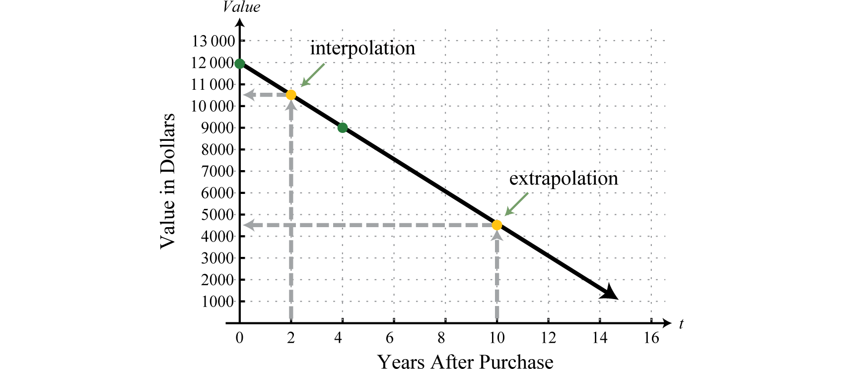
The function \(V (t) = −750t + 12,000\) called a linear depreciation model36. It uses a linear equation to expresses the declining value of an item over time. Using this function to determine the value of the item between the given data points is called interpolation37. For example, we can use the function to determine the value of the item where \(t = 2\),
\(\begin{aligned} V ( 2 ) & = - 750 ( 2 ) + 12,000 \\ & = 10,500 \end{aligned}\)
The function shows that the item was worth \($10,500\) two years after it was purchased. Using this model to predict the value outside the given data points is called extrapolation38. For example, we can use the function to determine the value of the item when \(t = 10\):
\(\begin{aligned} V ( 10 ) & = - 750 ( 10 ) + 12,000 \\ & = - 7,500 + 12,000 \\ & = 4,500 \end{aligned}\)
The model predicts that the piece of equipment will be worth \($4,500\) ten years after it is purchased.
In a business application, revenue results from the sale of a number of items. For example, if an item can be sold for \($150\) and we let \(n\) represent the number of units sold, then we can form the following revenue function39:
\(R(n)=150n\)
Use this function to determine the revenue generated from selling \(n=100\) units,
\(R ( 100 ) = 150 ( 100 ) = 15,000\)
The function shows that the revenue generated from selling \(100\) items is \($15,000\). Typically, selling items does not represent the entire story. There are a number of costs associated with the generation of revenue. For example, if there is a one-time set up fee of \($5,280\) and each item cost \($62\) to produce, then we can form the following cost function40:
\(C ( n ) = 62 n + 5,280\)
Here \(n\) represents the number of items produced. Use this function to determine the cost associated with producing \(n = 100\) units:
\(C ( 100 ) = 62 ( 100 ) + 5,280 = 11,480\)
The function shows that the cost associated with producing 100 items is $11,480. Profit is revenue less costs:
\(\begin{aligned} \color{Cerulean} { Profit } & = \color {Cerulean} { Revenue -Cost } \\ & = 15,000 - 11,480 \\ & = 3,520 \end{aligned}\)
Therefore, the profit generated by producing and selling \(100\) items is \($3,520\). In general, given a revenue function \(R\) and a cost function \(C\), we can form a profit function41 by subtracting as follows:
\(P ( n ) = R ( n ) - C ( n )\)
Example \(\PageIndex{7}\):
The cost in dollars of producing n items is given by the formula \(C (n) = 62n + 5,280\). The revenue in dollars is given by \(R (n) = 150n\), where \(n\) represents the number items sold. Write a function that gives the profit generated by producing and selling n items. Use the function to determine how many items must be produced and sold in order to earn a profit of at least \($7,000\).
Solution
Obtain the profit function by subtracting the cost function from the revenue function.
\(\begin{aligned} P ( n ) & = R ( n ) - C ( n ) \\ & = 150 n - ( 62 n + 5,280 ) \\ & = 150 n - 62 n - 5,280 \\ & = 88 n - 5,280 \end{aligned}\)
Therefore, \(P (n) = 88n + 5,280\) models the profit. To determine the number of items that must be produced and sold to profit at least \($7,000\), solve the following:
\(\begin{aligned} P ( n ) & \geq 7,000 \\ 88 n - 5,280 & \geq 7,000 \\ 88 n & \geq 12,280 \\ n & \geq 139.5 \end{aligned}\)
Round up because the number of units produced and sold must be an integer. To see this, calculate the profit where \(n\) is \(139\) and \(140\) units.
\(\begin{array} { l } { P ( 139 ) = 88 ( 139 ) - 5,280 = 6,952 } \\ { P ( 140 ) = 88 ( 140 ) - 5,280 = 7,040 } \end{array}\)
Answer:
\(140\) or more items must be produced and sold in order to earn a profit of at least \($7,000\).
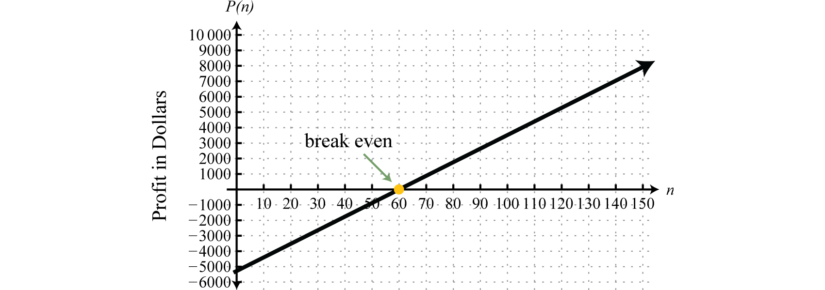
Sometimes the costs exceed the revenue, in which case, the profit will be negative. For example, use the profit function of the previous example, \(P (n) = 88n − 5,280\), to calculate the profit generated where \(n = 50\).
\(P ( 50 ) = 88 ( 50 ) - 5,280 = - 880\)
This indicates that when \(50\) units are produced and sold the corresponding profit is a loss of \($880\).
It is often important to determine how many items must be produced and sold to break even. To break even means to neither have a gain nor a loss; in this case, the profit will be equal to zero. To determine the breakeven point42, set the profit function equal to zero and solve:
\(\begin{aligned} P ( n ) & = 88 n - 5,280 \\ 0 & = 88 n - 5,280 \\ 5,280 & = 88 n \\ 60 & = n \end{aligned}\)
Therefore, \(60\) items must be produced and sold to break even.
Exercise \(\PageIndex{2}\)
Custom t-shirts can be sold for \($6.50\) each. In addition to an initial setup fee of \($120\), each t-shirt cost \($3.50\) to produce.
- Write a function that models the revenue and a function that models the cost.
- Determine a function that models the profit and use it to determine the profit from producing and selling \(150\) t-shirts.
- Calculate the number of t-shirts that must be sold to break even.
- Answer
-
a. Revenue: \(R (x) = 6.50x\); cost: \(C (x) = 3.50x + 120\);
b. profit: \(P (x) = 3x + 120\); \($330\)
c. \(40\)
Key Takeaways
- Given two points we can find the equation of a line.
- Parallel lines have the same slope.
- Perpendicular lines have slopes that are opposite reciprocals. In other words, if \(m = \frac{a}{b}\), then \(m_{⊥} = −\frac{b}{a}\).
- To find an equation of a line, first use the given information to determine the slope. Then use the slope and a point on the line to find the equation using point-slope form.
- To construct a linear function that models a real-world application, first identify the dependent and independent variables. Next, find two ordered pairs that describe the given situation. Use these two ordered pairs to construct a linear function by finding the slope and \(y\)-intercept.
Exercise \(\PageIndex{3}\)
Find the linear function \(f\) passing through the given points.
- \((−1, 2)\) and \((3, −4)\)
- \((3, −2)\) and \((−1, −4)\)
- \((−5, −6)\) and \((−4, 2)\)
- \((2, −7)\) and \((3, −5)\)
- \((10, −15)\) and \((7, −6)\)
- \((−9, 13)\) and \((−8, 12)\)
- \((−12, 22)\) and \((6, −20)\)
- \((6, −12)\) and \((−4, 13)\)
- \((\frac{1}{3}, \frac{4}{5})\) and \((\frac{1}{2} ,1)\)
- \((−\frac{3}{2}, −\frac{5}{2})\) and \((1, \frac{5}{6})\)
- \((−5, 10)\) and \((−1, 10)\)
- \((4, 0)\) and \((−7, 0)\)
- Answer
-
1. \(f (x) = −\frac{3}{2} x + \frac{1}{2}\)
3. \(f (x) = 8x + 34\)
5. \(f (x) = −3x + 15\)
7. \(f (x) = −\frac{7}{3} x − 6\)
9. \(f (x) = \frac{6}{5} x + \frac{2}{5}\)
11. \(f (x) = 10\)
Exercise \(\PageIndex{4}\)
Find the equation of the given linear function.
1.
2.
3.
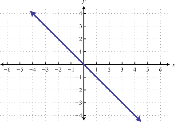
4.
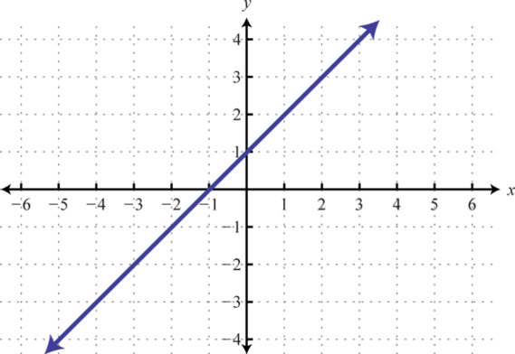
5.
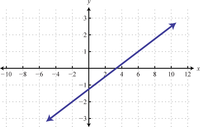
6.
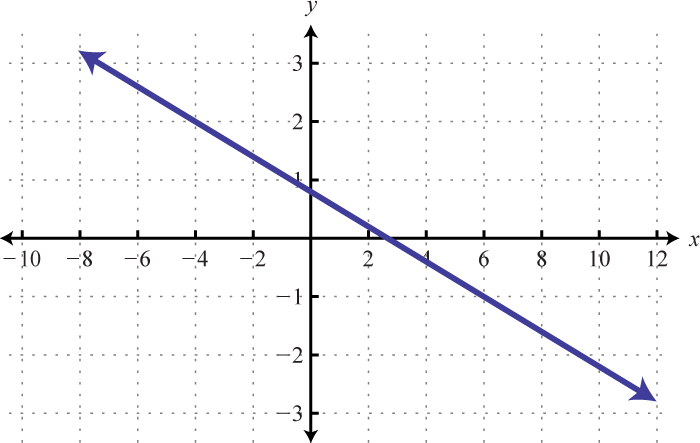
7.
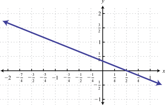
8.
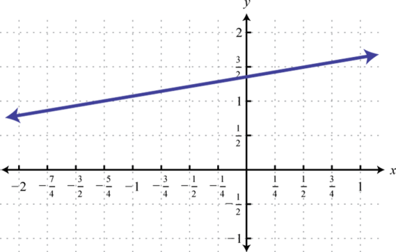
9.
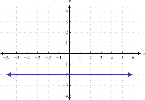
10.
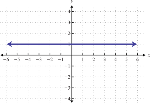
- Answer
-
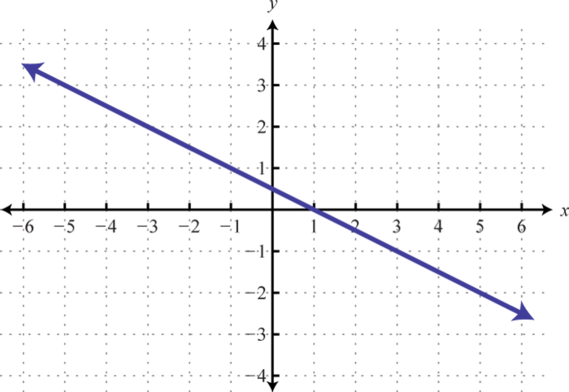
1. \(f (x) = − \frac{1}{2} x + \frac{1}{2}\)
3. \(f (x) = −x\)
5. \(f (x) = \frac{3}{8} x − \frac{5}{4}\)
7. \(f (x) = −\frac{2}{3} x + \frac{1}{3}\)
9. \(f (x) = −2\)
Exercise \(\PageIndex{5}\)
Find the equation of the line:
- Parallel to \(y = −\frac{5}{3}x +\frac{1}{2}\) and passing through \((−3, 4)\).
- Parallel to \(y = −\frac{3}{4}x −\frac{7}{3}\) and passing through \((−8, −1)\).
- Parallel to \(y = \frac{1}{3}x + 6\) and passing through \((2, −5)\).
- Parallel to \(y = \frac{1}{4}x + \frac{5}{3}\) and passing through \((5, 6)\).
- Parallel to \(4x − 5y = 15\) and passing through \((−1, −2)\).
- Parallel to \(3x − 4y = 2\) and passing through \((−6, 8)\).
- Parallel to \(2x + 12y = 9\) and passing through \((10, −9)\).
- Parallel to \(9x + 24y = 2\) and passing through \((−12, −4)\).
- Parallel to \(\frac{2}{15}x + \frac{1}{3}y = \frac{1}{10}\) and passing through \((−15, 4)\).
- Parallel to \(\frac{1}{3}x + \frac{2}{7}y = 1\) and passing through \((12, −11)\).
- Perpendicular to \(y = 5x + 2\) and passing through \((10, −5)\).
- Perpendicular to \(y = −2x + 1\) and passing through \((−8, −11)\).
- Perpendicular to \(y = \frac{3}{2}x − 5\) and passing through \((5, −3)\).
- Perpendicular to \(y = \frac{3}{4}x − \frac{1}{2}\) and passing through \((−6, −4)\).
- Perpendicular to \(12x + 15y = 3\) and passing through \((12, 15)\).
- Perpendicular to \(24x + 15y = 12\) and passing through \((2, −1)\).
- Perpendicular to \(14x − y = 3\) and passing through \((7, 3)\).
- Perpendicular to \(x − y = 4\) and passing through \((6, −2)\).
- Perpendicular to \(\frac{2}{15}x − \frac{3}{5}y = −1\) and passing through \((1, −1)\).
- Perpendicular to \(\frac{3}{4}x − \frac{2}{3}y = \frac{1}{2}\) and passing through \((−3, 6)\).
- Give the equation of the line that coincides with the \(x\)-axis.
- Give the equation of the line that coincides with the \(y\)-axis.
- Given any line in standard form, \(ax + by = c\), determine the slope of any perpendicular line.
- Given any line in standard form, \(ax + by = c\), determine the slope of any parallel line.
- Answer
-
1. \(y = −\frac{5}{3}x − 1\)
3. \(y = \frac{1}{3}x − \frac{17}{3}\)
5. \(y = \frac{4}{5}x − \frac{6}{5}\)
7. \(y = −\frac{1}{6}x − \frac{22}{3}\)
9. \(y = −\frac{2}{5}x − 2\)
11. \(y = −\frac{1}{5}x − 3\)
13. \(y = −\frac{2}{3}x + \frac{1}{3}\)
15. \(y = \frac{5}{4}x\)
17. \(y = −\frac{1}{14}x + \frac{7}{2}\)
19. \(y = −\frac{9}{2}x + \frac{7}{2}\)
21. \(y = 0\)
23. \(m_{⊥} = \frac{b}{a}\)
Exercise \(\PageIndex{6}\)
Use algebra to solve the following.
- A company wishes to purchase pens stamped with the company logo. In addition to an initial set-up fee of \($90\), each pen cost \($1.35\) to produce. Write a function that gives the cost in terms of the number of pens produced. Use the function to determine the cost of producing \(500\) pens with the company logo stamped on it.
- A rental car company charges a daily rate of \($42.00\) plus \($0.51\) per mile driven. Write a function that gives the cost of renting the car for a day in terms of the number of miles driven. Use the function to determine the cost of renting the car for a day and driving it \(76\) miles.
- A certain cellular phone plan charges \($16\) per month and \($0.15\) per minute of usage. Write a function that gives the cost of the phone per month based on the number of minutes of usage. Use the function to determine the number of minutes of usage if the bill for the first month was \($46\).
- A web-services company charges \($2.50\) a month plus \($0.14\) per gigabyte of storage on their system. Write a function that gives the cost of storage per month in terms of the number of gigabytes stored. How many gigabytes are stored if the bill for this month was \($6.00\)?
- Mary has been keeping track of her cellular phone bills for the last two months. The bill for the first month was \($45.00\) for \(150\) minutes of usage. The bill for the second month was \($25.00\) for \(50\) minutes of usage. Find a linear function that gives the total monthly bill based on the minutes of usage.
- A company in its first year of business produced \(1,200\) brochures for a total cost of \($5,050\). The following year, the company produced \(500\) more brochures at a cost of \($2,250\). Use this information to find a linear function that gives the total cost of producing brochures from the number of brochures produced.
- A Webmaster has noticed that the number of registered users has been steadily increasing since beginning an advertising campaign. Before starting to advertise, he had \(2,200\) registered users, and after \(4\) months of advertising he now has \(5,480\) registered users. Use this data to write a linear function that gives the total number of registered users, given the number of months after starting to advertise. Use the function to predict the number of users \(8\) months into the advertising campaign.
- A corn farmer in California was able to produce \(154\) bushels of corn per acre \(2\) years after starting his operation. Currently, after \(7\) years of operation, he has increased his yield to \(164\) bushels per acre. Use this information to write a linear function that gives the total yield per acre based on the number of years of operation, and use it to predict the yield for next year.
- A commercial van was purchased new for \($22,500\) and is expected to be worthless in \(12\) years. Use this information to write a linear depreciation function for the value of the van. Use the function to determine the value of the van after \(8\) years of use.
- The average lifespan of an industrial welding robot is \(10\) years, after which it is considered to have no value. If an industrial welding robot was purchased new for \($58,000\), write a function that gives the value of the robot in terms of the number of years of operation. Use the function to value the robot after \(3\) years of operation.
- A business purchased a piece of equipment new for \($2,400\). After \(5\) years of use the equipment is valued at \($1,650\). Find a linear function that gives the value of the equipment in terms of years of usage. Use the function to determine the number of years after which the piece of equipment will have no value.
- A salesman earns a base salary of \($2,400\) a month plus a \(5\)% commission on all sales. Write a function that gives the salesman’s monthly salary in terms of sales. Use the function to determine the monthly sales required to earn at least \($3,600\) a month.
- When a certain professor was hired in \(2005\), the enrollment at a college was \(8,500\) students. Five years later, in \(2010\), the enrollment grew to \(11,200\) students. Determine a linear growth function that models the student population in years since \(2005\). Use the model to predict the year in which enrollment will exceed \(13,000\) students.
- In \(1980\), the population of California was about \(24\) million people. Twenty years later, in the year \(2000\), the population was about \(34\) million. Use this data to construct a linear function to model the population growth in years since \(1980\). Use the function to predict the year in which the population will reach \(40\) million.
- A classic car is purchased for \($24,500\) and is expected to increase in value each year by \($672\). Write a linear function that models the appreciation of the car in terms of the number of years after purchase. Use the function to predict the value of the car in \(7\) years.
- A company reported first and second quarter sales of \($52,000\) and \($64,500\), respectively.
- Write a linear function that models the sales for the year in terms of the quarter \(n\).
- Use the model to predict the sales in the third and fourth quarters.
- A particular search engine assigns a ranking to a webpage based on the number of links that direct users to the webpage. If no links are found, the webpage is assigned a ranking of \(1\). If \(20\) links are found directing users to the webpage, the search engine assigns a page ranking of \(3.5\).
- Find a linear function that gives the webpage ranking based on the number of links that direct users to it.
- How many links will be needed to obtain a page ranking of \(5\)?
- Online sales of a particular product are related to the number of clicks on its advertisement. It was found that \(1,520\) clicks in a month results in \($2,748\) of online sales, and that \(1,840\) clicks results in \($2,956\) of online sales. Write a linear function that models the online sales of the product based on the number of clicks on its advertisement. How many clicks would we need to expect \($3,385\) in monthly online sales from this particular product?
- A bicycle manufacturing business can produce \(x\) bicycles at a cost, in dollars, given by the formula \(C (x) = 85x + 2,400\). The company sells each bicycle at a wholesale price of \($145\). The revenue, in dollars, is given by \(R (x) = 145x\), where \(x\) represents the number of bicycles sold. Write a function that gives profit in terms of the number of bicycles produced and sold. Use the function to determine the number of bicycles that need to be produced and sold to break even.
- The cost, in dollars, of producing \(n\) custom lamps is given by the formula \(C (n) = 28n + 360\). Each lamp can be sold online for \($79\). The revenue in dollars, is given by \(R (n) = 79n\), where \(n\) represents the number of lamps sold. Write a function that gives the profit from producing and selling \(n\) custom lamps. Use the function to determine how many lamps must be produced and sold to earn at least \($1,000\) in profit.
- A manufacturer can produce a board game at a cost of \($12\) per unit after an initial fixed retooling investment of \($12,500\). The games can be sold for \($22\) each to retailers.
- Write a function that gives the manufacturing costs when \(n\) games are produced.
- Write a function that gives the revenue from selling \(n\) games to retailers.
- Write a function that gives the profit from producing and selling \(n\) units.
- How many units must be sold to earn a profit of at least \($37,500\)?
- A vending machine can be leased at a cost of \($90\) per month. The items used to stock the machine can be purchased for \($0.50\) each and sold for \($1.25\) each.
- Write a function that gives the monthly cost of leasing and stocking the vending machine with \(n\) items.
- Write a function that gives the revenue generated by selling \(n\) items.
- Write a function that gives the profit from stocking and selling \(n\) items per month.
- How many items must be sold each month to break even?
- Answer
-
1. \(C ( x ) = 1.35 x + 90 ; \$ 765\)
3. \(C ( x ) = 0.15 x + 16 ;\: 200 \:\text{minutes}\)
5. \(C ( x ) = 0.20 x + 15\)
7. \(U ( x ) = 820 x + 2,200 \:; 8,760 \: \text{users}\)
9. \(V ( t ) = - 1,875 t + 22,500 ;\: \$ 7,500\)
11. \(V ( t ) = - 150 t + 2,400\: ; 16\: \text{years}\)
13. \(P ( x ) = 540 x + 8,500 ;\: 2013\)
15. \(V ( t ) = 672 t + 24,500 ;\: \$ 29,204\)
17. (1) \(r ( n ) = 0.125 n + 1\); (2) \(32\) links
19. \(P ( x ) = 60 x - 2,400\: ; 40\:\text{bicycles}\)
21. (1) \(C ( n ) = 12 n + 12,500\); (2) \(R ( n ) = 22 n\); (3) \(P ( n ) = 10 n - 12,500\); (4) at least \(5,000\) units
Exercise \(\PageIndex{1}\)
- Research and discuss linear depreciation. In a linear depreciation model, what do the slope and \(y\)-intercept represent?
- Write down your own steps for finding the equation of a line. Post your steps on the discussion board.
- Answer
-
1. Answer may vary
Footnotes
30Any nonvertical line can be written in the form \(y − y_{1} = m (x − x_{1} )\), where \(m\) is the slope and \((x_{1} , y_{1} )\) is any point on the line.
31Lines in the same plane that do not intersect; their slopes are the same.
32Lines in the same plane that intersect at right angles; their slopes are opposite reciprocals.
33Used when referring to opposite reciprocals.
34Two real numbers whose product is \(−1\). Given a real number \(\frac{a}{b}\), the opposite reciprocal is \(−\frac{b}{a}\).
35Using data to find mathematical equations that describe, or model, real-world applications.
36A linear function used to describe the declining value of an item over time.
37Using a linear function to estimate a value between given data points.
38Using a linear function to estimate values that extend beyond the given data points.
39A function that models income based on a number of units sold.
40A function that models the cost of producing a number of units.
41A function that models the profit as revenue less cost.
42The point at which profit is neither negative nor positive; profit is equal to zero.


